4 Discriminant Analysis

Discriminant analysis is a popular method for multiple-class classiﬁcation. We will start first by the Linear Discriminant Analysis (LDA).

4.1 Introduction

As we saw in the previous chapter, Logistic regression involves directly modeling \(\mathbb{P} (Y = k|X = x)\) using the logistic function, for the case of two response classes. In logistic regression, we model the conditional distribution of the response \(Y\), given the predictor(s) \(X\). We now consider an alternative and less direct approach to estimating these probabilities. In this alternative approach, we model the distribution of the predictors \(X\) separately in each of the response classes (i.e. given \(Y\)), and then use Bayes’ theorem to flip these around into estimates for \(\mathbb{P} (Y = k|X = x)\). When these distributions are assumed to be Normal, it turns out that the model is very similar in form to logistic regression.

Why not logistic regression? Why do we need another method, when we have logistic regression? There are several reasons:

When the classes are well-separated, the parameter estimates for the logistic regression model are surprisingly unstable. Linear discriminant analysis does not suﬀer from this problem.
If \(n\) is small and the distribution of the predictors \(X\) is approximately normal in each of the classes, the linear discriminant model is again more stable than the logistic regression model.
Linear discriminant analysis is popular when we have more than two response classes.

4.2 Bayes’ Theorem

Bayes’ theorem is stated mathematically as the following equation:

\[ P(A | B) = \frac{P(A \cap B)}{P(B)} = \frac{P(B|A) P(A)}{P(B)}\]

where \(A\) and \(B\) are events and \(P(B) \neq 0\).

\(P(A | B)\), a conditional probability, is the probability of observing event \(A\) given that \(B\) is true. It is called the posterior probability.
\(P(A)\), is called the prior, is the initial degree of belief in A.
\(P(B)\) is the likelihood.

The posterior probability can be written in the memorable form as :

Posterior probability \(\propto\) Likelihood \(\times\) Prior probability.

Extended form:

Suppose we have a partition \(\{A_i\}\) of the sample space, the even space is given or conceptualized in terms of \(P(A_j)\) and \(P(B | A_j)\). It is then useful to compute \(P(B)\) using the law of total probability:

\[ P(B) = \sum_j P(B|A_j) P(A_j) \]

\[ \Rightarrow P(A_i|B) = \frac{P(B|A_i) P(A_i)}{\sum_j P(B|A_j) P(A_j)} \]

Bayes’ Theorem for Classification:

Suppose that we wish to classify an observation into one of \(K\) classes, where \(K \geq 2\). In other words, the qualitative response variable \(Y\) can take on \(K\) possible distinct and unordered values.

Let \(\pi_k\) represent the overall or prior probability that a randomly chosen observation comes from the \(k\)-th class; this is the probability that a given observation is associated with the \(k\)-th category of the response variable \(Y\).

Let \(f_k(X) \equiv P(X = x|Y = k)\) denote the density function of \(X\) for an observation that comes from the \(k\)-th class. In other words, \(f_k(x)\) is relatively large if there is a high probability that an observation in the \(k\)-th class has \(X \approx x\), and \(f_k(x)\) is small if it is very unlikely that an observation in the \(k\)-th class has \(X \approx x\). Then Bayes’ theorem states that

\[\begin{equation} P(Y=k|X=x) = \frac{ \pi_k f_k(x)}{\sum_{c=1}^K \pi_c f_c(x)} \tag{4.1} \end{equation}\]

As we did in the last chapter, we will use the abbreviation \(p_k(X) =P(Y = k|X)\).

The equation above stated by Bayes’ theorem suggests that instead of directly computing \(p_k(X)\) as we did in the logistic regression, we can simply plug in estimates of \(\pi_k\) and \(f_k(X)\) into the equation. In general, estimating \(\pi_k\) is easy (the fraction of the training observations that belong to the \(k\)-th class). But estimating \(f_k(X)\) tends to be more challenging.

Recall that \(p_k(x)\) is the posterior probability that an observation \(X=x\) belongs to \(k\)-th class.

If we can find a way to estimate \(f_k(X)\), we can develop a classifier with the lowest possibe error rate out of all classifiers.

4.3 LDA for \(p=1\)

Assume that \(p=1\), which mean we have only one predictor. We would like to obtain an estimate for \(f_k(x)\) that we can plug into the Equation (4.1) in order to estimate \(p_k(x)\). We will then classify an observation to the class for which \(p_k(x)\) is greatest.

In order to estimate \(f_k(x)\), we will first make some assumptions about its form.

Suppose we assume that \(f_k(x)\) is normal (Gaussian). In the one-dimensional setting, the normal density take the form

\[\begin{equation} f_k(x)= \frac{1}{\sigma_k\sqrt{2\pi}} \exp \big( - \frac{1}{2\sigma_k^2 } (x-\mu_k)^2\big) \tag{4.2} \end{equation}\]

where \(\mu_k\) and \(\sigma_k^2\) are the mean and variance parameters for \(k\)-th class. Let us assume that \(\sigma_1^2 = \ldots = \sigma_K^2 = \sigma^2\) (which means there is a shared variance term across all \(K\) classes). Plugging Eq. (4.2) into the Bayes formula in Eq. (4.1) we get,

\[\begin{equation} p_k(x) = \frac{ \pi_k \frac{1}{\sigma \sqrt{2\pi}} e^{-\frac{1}{2} \big(\frac{x-\mu_k}{\sigma}\big)^2 } }{ \sum_{c=1}^K \pi_c \frac{1}{\sigma \sqrt{2\pi}} e^{-\frac{1}{2} \big(\frac{x-\mu_c}{\sigma}\big)^2 } } \tag{4.3} \end{equation}\]

Note that \(\pi_k\) and \(\pi_c\) denote the prior probabilities. And \(\pi\) is the mathematical constant \(\pi \approx 3.14159\).

To classify at the value \(X = x\), we need to see which of the \(p_k(x)\) is largest. Taking logs, and discarding terms that do not depend on \(k\), we see that this is equivalent to assigning \(x\) to the class with the largest discriminant score:

\[\begin{equation} \delta_k(x) = x.\frac{\mu_k}{\sigma^2} - \frac{\mu_k^2}{2\sigma^2} + \log (\pi_k) \tag{4.4} \end{equation}\]

Note that \(\delta_k(x)\) is a linear function of \(x\).

The decision surfaces (e.g. decision boundaries) for a linear discriminant classifiers are defined by the linear equations \(\delta_k(x) = \delta_c(x)\), for all classes \(k\neq c\). It represents the set of values \(x\) for which the probability of belonging to classes \(k\) and \(c\) is the same, \(0.5\).
Example: If \(K=2\) and \(\pi_1=\pi_2\), then the desicion boundary is at \(x=\frac{\mu_1+\mu2}{2}\) (Prove it!).
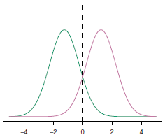
An example where \(\mu_1=-1.5\), \(\mu_2=1.5\), \(\pi_1=\pi_2=0.5\) and \(\sigma^2=1\) is shown in this following figure

See this video to understand more about decision boundary (Applied on logistic regression).
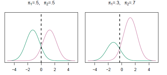
As we classify a new point according to which density is highest, when the priors are diﬀerent we take them into account as well, and compare \(\pi_k f_k(x)\). On the right of the following figure, we favor the pink class (remark that the decision boundary has shifted to the left).

4.4 Estimating the parameters

Typically we don’t know these parameters; we just have the training data. In that case we simply estimate the parameters and plug them into the rule.

Let \(n\) the total number of training observations, and \(n_k\) the number of training observations in the \(k\)-th class. The following estimates are used:

\[\begin{align*} \hat{\pi}_k &= \frac{n_k}{n} \\ \hat{\mu}_k &= \frac{1}{n_k} \sum_{i: y_i=k} x_i \\ \hat{\sigma}^2 &= \frac{1}{n - K} \sum_{k=1}^K \sum_{i: y_i=k} (x_i-\hat{\mu}_k)^2 \\ &= \sum_{k=1}^K \frac{n_k-1}{n - K} . \hat{\sigma}_k^2 \end{align*}\]

where \(\hat{\sigma}_k^2 = \frac{1}{n_k-1}\sum_{i: y_i=k}(x_i-\hat{\mu}_k)^2\) is the usual formula for the estimated variance in the -\(k\)-th class.

The linear discriminant analysis (LDA) classifier plugs these estimates in Eq. (4.4) and assigns an observation \(X=x\) to the class for which

\[\begin{equation} \hat{\delta}_k(x) = x.\frac{\hat{\mu}_k}{\hat{\sigma}^2} - \frac{\hat{\mu}_k^2}{2\hat{\sigma}^2} + \log (\hat{\pi}_k) \tag{4.5} \end{equation}\]

is largest.

The discriminant functions in Eq. (4.5) are linear functions of \(x\).

Recall that we assumed that the observations come from a normal distribution with a common variance \(\sigma^2\).

4.5 LDA for \(p > 1\)

Let us now suppose that we have multiple predictors. We assume that \(X=(X_1,X_2,\ldots,X_p)\) is drawn from multivariate Gaussian distribution (assuming they have a common covariance matrix, e.g. same variances as in the case of \(p=1\)). The multivariate Gaussian distribution assumes that each individual predictor follows a one-dimensional normal distribution as in Eq. (4.2), with some correlation between each pair of predictors.

To indicate that a \(p\)-dimensional random variable \(X\) has a multivariate Gaussian distribution, we write \(X \sim \mathcal{N}(\mu,\Sigma)\). Where

\[ \mu = E(X) = \begin{pmatrix} \mu_1 \\ \mu_2 \\ \vdots \\ \mu_p \end{pmatrix} \]

and, \[ \Sigma = Cov(X) = \begin{pmatrix} \sigma_1^2 & Cov[X_1, X_2] & \dots & Cov[X_1, X_p] \\ Cov[X_2, X_1] & \sigma_2^2 & \dots & Cov[X_2, X_p] \\ \vdots & \vdots & \ddots & \vdots \\ Cov[X_p, X_1] & Cov[X_p, X_2] & \dots & \sigma_p^2 \end{pmatrix} \]

\(\Sigma\) is the \(p\times p\) covariance matrix of \(X\).

Formally, the multivariate Gaussian density is deﬁned as

\[f(x) = \frac{1}{(2\pi)^{p/2} |\Sigma|^{1/2}} \exp \bigg( - \frac{1}{2} (x-\mu)^T \Sigma^{-1} (x-\mu) \bigg) \]

Plugging the density function for the \(k\)-th class, \(f_k(X=x)\), into Eq. (4.1) reveals that the Bayes classifier assigns an observation \(X=x\) to the class for which

\[\begin{equation} \delta_k(x) = x^T \Sigma^{-1} \mu_k - \frac{1}{2} \mu_k^T \Sigma^{-1} \mu_k + \log \pi_k \tag{4.6} \end{equation}\]

is largest. This is the vector/matrix version of (4.4).

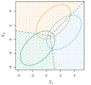
An example is shown in the following figure. Three equally-sized Gaussian classes are shown with class-specific mean vectors and a common covariance matrix (\(\pi_1=\pi_2=\pi_3=1/3\)). The three ellipses represent regions that contain \(95\%\) of the probability for each of the three classes. The dashed lines are the Bayes decision boundaries.

Recall that the decision boundaries represent the set of values \(x\) for which \(\delta_k(x)=\delta_c(x)\); i.e. for \(k\neq c\).

\[ x^T \Sigma^{-1} \mu_k - \frac{1}{2} \mu_k^T \Sigma^{-1} \mu_k = x^T \Sigma^{-1} \mu_c - \frac{1}{2} \mu_c^T \Sigma^{-1} \mu_c \]

Note that there are three lines representing the Bayes decision boundaries because there are three pairs of classes among the three classes. That is, one Bayes decision boundary separates class 1 from class 2, one separates class 1 from class 3, and one separates class 2 from class 3. These three Bayes decision boundaries divide the predictor space into three regions. The Bayes classiﬁer will classify an observation according to the region in which it is located.

Once again, we need to estimate the unknown parameters \(\mu_1,\ldots,\mu_k,\) and \(\pi_1,\ldots,\pi_k,\) and \(\Sigma\); the formulas are similar to those used in the one-dimensional case. To assign a new observation \(X = x\), LDA plugs these estimates into Eq. (4.6) and classiﬁes to the class for which \(\delta_k(x)\) is largest.

Note that in Eq. (4.6) \(\delta_k(x)\) is a linear function of \(x\); that is, the LDA decision rule depends on \(x\) only through a linear combination of its elements (e.g. the decision boundaries are linear). This is the reason for the word linear in LDA.

4.6 Making predictions

Once we have estimates \(\hat{\delta}_k(x)\), we can turn these into estimates for class probabilities:

\[ \hat{P}(Y=k|X=x)= \frac{e^{\hat{\delta}_k(x)}}{\sum_{c=1}^K e^{\hat{\delta}_c(x)}} \]

So classifying to the largest \(\hat{\delta}_k(x)\) amounts to classifying to the class for which \(\hat{P}(Y=k|X=x)\) is largest.

When \(K=2\), we classify to class 2 if \(\hat{P}(Y=2|X=x) \geq 0.5\), else to class \(1\).

4.7 Other forms of Discriminant Analysis

\[P(Y=k|X=x) = \frac{ \pi_k f_k(x)}{\sum_{c=1}^K \pi_c f_c(x)}\]

We saw before that when \(f_k(x)\) are Gaussian densities, whith the same covariance matrix \(\Sigma\) in each class, this leads to Linear Discriminant Analysis (LDA).

By altering the forms for \(f_k(x)\), we get different classifiers.

With Gaussians but different \(\Sigma_k\) in each class, we get Quadratic Discriminant Analysis (QDA).
With \(f_k(x) = \prod_{j=1}^p f_{jk}(x_j)\) (conditional independence model) in each class we get Naive Bayes. (For Gaussian, this mean the \(\Sigma_k\) are diagonal, e.g. \(Cov(X_i,X_j)=0 \,\, \forall \, \, 1\leq i,j \leq p\)).
Many other forms by proposing specific density models for \(f_k(x)\), including nonparametric approaches.

4.7.1 Quadratic Discriminant Analysis (QDA)

Like LDA, the QDA classiﬁer results from assuming that the observations from each class are drawn from a Gaussian distribution, and plugging estimates for the parameters into Bayes’ theorem in order to perform prediction.

However, unlike LDA, QDA assumes that each class has its own covariance matrix. Under this assumption, the Bayes classiﬁer assigns an observation \(X = x\) to the class for which

\[\begin{align*} \delta_k(x) &= - \frac{1}{2} (x-\mu)^T \Sigma_k^{-1} (x-\mu) - \frac{1}{2} \log |\Sigma_k| + \log \pi_k \\ &= - \frac{1}{2} x^T \Sigma_k^{-1} x + \frac{1}{2} x^T \Sigma_k^{-1} \mu_k - \frac{1}{2} \mu_k^T \Sigma_k^{-1} \mu_k - \frac{1}{2} \log |\Sigma_k| + \log \pi_k \end{align*}\]

is largest.

Unlike in LDA, the quantity \(x\) appears as a quadratic function in QDA. This is where QDA gets its name.

The decision boundary in QDA is non-linear. It is quadratic (a curve).

4.7.2 Naive Bayes

We use Naive Bayes classifier if the features are independant in each class. It is useful when \(p\) is large (unklike LDA and QDA).

Naive Bayes assumes that each \(\Sigma_k\) is diagonal, so

\[\begin{align*} \delta_k(x) &\propto \log \bigg[\pi_k \prod_{j=1}^p f_{kj}(x_j) \bigg] \\ &= -\frac{1}{2} \sum_{j=1}^p \frac{(x_j-\mu_{kj})^2}{\sigma_{kj}^2} + \log \pi_k \end{align*}\]

It can used for mixed feature vectors (qualitative and quantitative). If \(X_j\) is qualitative, we replace \(f_{kj}(x_j)\) by probability mass function (histogram) over discrete categories.

4.8 LDA vs Logistic Regression

the logistic regression and LDA methods are closely connected. Consider the two-class setting with \(p =1\) predictor, and let \(p_1(x)\) and \(p_2(x)=1−p_1(x)\) be the probabilities that the observation \(X = x\) belongs to class 1 and class 2, respectively. In the LDA framework, we can see from Eq. (4.4) (and a bit of simple algebra) that the log odds is given by

\[ \log \bigg(\frac{p_1(x)}{1-p_1(x)}\bigg) = \log \bigg(\frac{p_1(x)}{p_2(x)}\bigg) = c_0 + c_1 x\]

where \(c_0\) and \(c_1\) are functions of \(\mu_1, \mu_2,\) and \(\sigma^2\).

On the other hand, we know that in logistic regression

\[ \log \bigg(\frac{p_1}{1-p_1}\bigg) = \beta_0 + \beta_1 x\]

Both of the equations above are linear functions of \(x\). Hence both logistic regression and LDA produce linear decision boundaries. The only diﬀerence between the two approaches lies in the fact that \(\beta_0\) and \(\beta_1\) are estimated using maximum likelihood, whereas \(c_0\) and \(c_1\) are computed using the estimated mean and variance from a normal distribution. This same connection between LDA and logistic regression also holds for multidimensional data with \(p> 1\).

Logistic regression uses the conditional likelihood based on \(P(Y|X)\) (known as discriminative learning).
LDA uses the full likelihood based on \(P(X,Y )\) (known as generative learning).
Despite these differences, in practice the results are often very similar.

Remark: Logistic regression can also fit quadratic boundaries like QDA, by explicitly including quadratic terms in the model.

◼

PW 3

PW 4