2 Multiple Linear Regression

Simple linear regression is a useful approach for predicting a response on the basis of a single predictor variable. However, in practice we often have more than one predictor. In the previous chapter, we took for example the prediction of housing prices considering we had the size of each house. We had a single feature \(X\), the size of the house. But now imagine if we had not only the size of the house as a feature but we also knew the number of bedrooms, the number of flours and the age of the house in years. It seems like this would give us a lot more information with which to predict the price.

2.1 The Model

In general, suppose that we have \(p\) distinct predictors. Then the multiple linear regression model takes the form

\[ Y = \beta_0 + \beta_1 X_1 + \beta_2 X_2 + \dots + \beta_p X_p + \epsilon \]

where \(X_j\) represents the \(j\)th predictor and \(\beta_j\) quantifies the association between that variable and the response. We interpret \(\beta_j\) as the average effect on \(Y\) of a one unit increase in \(X_j\), holding all other predictors fixed.

In matrix terms, supposing we have \(n\) observations and \(p\) variables, we need to define the following matrices:

\[\begin{equation} \textbf{Y}_{n \times 1} = \begin{pmatrix} Y_{1} \\ Y_{2} \\ \vdots \\ Y_{n} \end{pmatrix} \,\,\,\,\,\,\,\,\,\,\,\, \textbf{X}_{n \times (p+1)} = \begin{pmatrix} 1 & X_{11} & X_{12} & \dots & X_{1p} \\ 1 & X_{21} & X_{22} & \dots & X_{2p} \\ \vdots & \vdots & \vdots & \ddots & \vdots \\ 1 & X_{n1} & X_{n2} & \dots & X_{np} \end{pmatrix} \end{equation}\]

\[\begin{equation} {\mathbb{\beta}}_{(p+1) \times 1} = \begin{pmatrix} \beta_{0} \\ \beta_{1} \\ \vdots \\ \beta_{p} \end{pmatrix} \,\,\,\,\,\,\,\,\,\,\,\, {\epsilon}_{n \times 1} = \begin{pmatrix} \epsilon_{1} \\ \epsilon_{2} \\ \vdots \\ \epsilon_{n} \end{pmatrix} \end{equation}\]

In matrix terms, the general linear regression model is

\[ \textbf{Y}_{n \times 1} = \textbf{X}_{n \times (p+1)} {\mathbb{\beta}}_{(p+1) \times 1} + {\epsilon}_{n \times 1} \]

where,

• \(\textbf{Y}\) is a vector of responses.
• \(\mathbb{\beta}\) is a vector of parameters.
• \(\textbf{X}\) is a matrix of constants.
• \(\epsilon\) is a vector of independent normal (Gaussian) random variables.

2.2 Estimating the Regression Coefficients

As was the case in the simple linear regression setting, the regression coefficients \(\beta_{0}, \beta_{1}, \ldots, \beta_{p}\) are unknown, and must be estimated. Given estimates \(\hat{\beta_{0}}, \hat{\beta_{1}}, \ldots, \hat{\beta_{p}}\), we can make predictions using the formula

\[ \hat{y} = \hat{\beta_{0}} + \hat{\beta_{1}} x_1 + \hat{\beta_{2}} x_2 + \ldots + \hat{\beta_{p}} x_p \]

We choose \(\beta_{0}, \beta_{1}, \ldots, \beta_{p}\) to minimize the residual sum of squares

\[ \begin{aligned} RSS &= \sum_{i=1}^{n} (y_i - \hat{y}_i)^2 \\ &= \sum_{i=1}^{n} (y_i - \hat{\beta_0} - \hat{\beta_1} {x}_{i1} - \hat{\beta_2} {x}_{i2} - \ldots - \hat{\beta_p} {x}_{ip})^2 \\ \end{aligned} \]

The values \(\hat{\beta_{0}}, \hat{\beta_{1}}, \ldots, \hat{\beta_{p}}\) that minimize the RSS are the multiple least squares regression coefficient estimates, they are calculated using this formula (in matrix terms):

\[ \hat{\beta} = (\textbf{X}^T \textbf{X})^{-1}\textbf{X}^T \textbf{Y} \]

To obtain \(\hat{\beta}\), we can write the residual sum of squares as

\[ RSS = (\textbf{Y}-\textbf{X}\beta)^T(\textbf{Y}-\textbf{X}\beta) \]

This is a quadratic function in the \(p+1\) parameters. Differentiating with respect to \(\beta\) we obtain \[ \begin{aligned} \frac{\partial RSS}{\partial \beta} &= -2\textbf{X}^T(\textbf{Y}-\textbf{X}\beta) \\ \frac{\partial^2 RSS}{\partial \beta \partial \beta^T} &= 2\textbf{X}^T\textbf{X}.\\ \end{aligned} \]

Assuming (for the moment) that \(\textbf{X}\) has full column rank, and hence \(\textbf{X}^T\textbf{X}\) is positive definite⁷, we set the first derivative to zero

\[\textbf{X}^T(\textbf{Y}-\textbf{X}\beta)=0\] to obtain the unique solution

\[ \hat{\beta} = (\textbf{X}^T \textbf{X})^{-1}\textbf{X}^T \textbf{Y} \]

Note 1:

It is a remarkable property of matrix algebra that the results for the general linear regression model in matrix notation appear exactly as those for the simple linear regression model. Only the degrees of freedom and other constants related to the number of \(X\) variables and the dimensions of some matrices are different. Which means there are some similarities between \(\hat{\beta} = (\textbf{X}^T \textbf{X})^{-1}\textbf{X}^T \textbf{Y}\) and \(\hat\beta_1=(s_x^2)^{-1}s_{xy}\) from the simple linear model: both are related to the covariance between \(\mathbf{X}\) and \(\mathbf{Y}\) weighted by the variance of \(\mathbf{X}\).

Note 2:

If \(\textbf{X}^T \textbf{X}\) is noninvertible, the common causes might be having:

• Redundant features, where two features are very closely related (i.e. they are linearly dependent)
• Too many features (e.g. \(p \geq n\)). In this case, we delete some features or we use “regularization” (to be, maybe, explained in a later lesson).

2.3 Some important questions

When we perform multiple linear regression, we usually are interested in answering a few important questions.

1. Is at least one of the predictors \(X_1 ,X_2 ,\ldots,X_p\) useful in predicting the response?
2. Do all the predictors help to explain \(Y\), or is only a subset of the predictors useful?
3. How well does the model fit the data?
4. Given a set of predictor values, what response value should we predict, and how accurate is our prediction?

Relationship Between the Response and Predictors?

\(F\)-Statistic

Recall that in the simple linear regression setting, in order to determine whether there is a relationship between the response and the predictor we can simply check whether \(\beta_1 = 0\). In the multiple regression setting with \(p\) predictors, we need to ask whether all of the regression coefficients are zero, i.e. whether \(\beta_1 = \beta_2 = \ldots = \beta_p = 0\). As in the simple linear regression setting, we use a hypothesis test to answer this question. We test the null hypothesis,

\[ H_0 : \beta_1 = \beta_2 = \ldots = \beta_p = 0 \]

versus the alternative hypothesis

\[ H_1 : \text{at least one} \, \beta_j \, \text{is non-zero} \]

This hypothesis test is performed by computing the \(F\)-statistic (Fisher):

\[ F = \frac{ (\text{TSS} - \text{RSS})/p}{\text{RSS}/(n-p-1)} \sim F_{p,n-p-1} \]

where, as with simple linear regression, \(\text{TSS} = \sum (y_i - \bar{y})^2\) and \(\text{RSS} = \sum (y_i - \hat{y}_i)^2\).

Note that \(F_{p,n-p-1}\) represents the Fisher-Snedecor’s \(F\) distribution with \(p\) and \(n-p-1\) degrees of freedom. If \(H_0\) is true, then \(F\) is expected to be small since ESS⁸ will be close to zero (little variation is explained by the regression model since \(\hat{\boldsymbol{\beta}}\approx\mathbf{0}\)).

So the question we ask here: Is the whole regression explaining anything at all? The answer comes from the \(F\)-test in the ANOVA (ANalysis Of VAriance) table. This is what we get in an ANOVA table:

Source	df	SS	MS	\(F\)	p-value
Factor (Explained)	\(p\)	ESS=SSR	MSR=ESS/\((p)\)	F=MSR/MSE	p-value
Error (Unexplained)	\(n-p-1\)	RSS=SSE	MSE=RSS/\((n-p-1)\)
Total	\(n-1\)	TSS=SST

The ANOVA table has many pieces of information. What we care about is the \(F\) Ratio and the corresponding p-value. We compare the \(F\) Ratio with \(F_{(p,n-p-1)}\) and a corresponding \(\alpha\) value (error).

The “ANOVA table” is a broad concept in statistics, with different variants. Here we are only covering the basic ANOVA table from the relation \(\text{SST} = \text{SSR} + \text{SSE}\). However, further sophistications are possible when \(\text{SSR}\) is decomposed into the variations contributed by each predictor. In particular, for multiple linear regression r fontawesome::fa(“r-project”, fill =“steelblue”)’s anova implements a sequential (type I) ANOVA table, which is not the previous table!

The anova function in takes a model as an input and returns the following sequential ANOVA table⁹:

	Degrees of freedom	Sum Squares	Mean Squares	\(F\)-value	\(p\)-value
Predictor 1	\(1\)	ESS\(_1\)	\(\frac{\text{ESS}_1}{1}\)	\(\frac{\text{ESS}_1/1}{\text{RSS}/(n-p-1)}\)	\(p_1\)
Predictor 2	\(1\)	ESS\(_2\)	\(\frac{\text{ESS}_2}{1}\)	\(\frac{\text{ESS}_2/1}{\text{RSS}/(n-p-1)}\)	\(p_2\)
\(\vdots\)	\(\vdots\)	\(\vdots\)	\(\vdots\)	\(\vdots\)	\(\vdots\)
Predictor \(p\)	\(1\)	ESS\(_p\)	\(\frac{\text{ESS}_p}{1}\)	\(\frac{\text{ESS}_p/1}{\text{RSS}/(n-p-1)}\)	\(p_p\)
Residuals	\(n - p - 1\)	RSS	\(\frac{\text{RSS}}{n-p-1}\)

Here the ESS\(_j\) represents the explained sum of squares (same as regression sum of squares) associated to the inclusion of \(X_j\) in the model with predictors \(X_1,\ldots,X_{j-1}\), this is: \[ \text{ESS}_j=\text{ESS}(X_1,\ldots,X_j)-\text{ESS}(X_1,\ldots,X_{j-1}). \] The \(p\)-values \(p_1,\ldots,p_p\) correspond to the testing of the hypotheses \[\begin{align*} H_0:\beta_j=0\quad\text{vs.}\quad H_1:\beta_j\neq 0, \end{align*}\] carried out inside the linear model \(Y=\beta_0+\beta_1X_1+\ldots+\beta_jX_j+\varepsilon\). This is like the \(t\)-test for \(\beta_j\) for the model with predictors \(X_1,\ldots,X_j\). Recall that there is no \(F\)-test in this version of the ANOVA table.

p-values

The p-values provide information about whether each individual predictor is related to the response, after adjusting for the other predictors. Let’s look at the following table we obtain in general using a statistical software for example

	Coefficient	Std. error	\(t\)-statistic	p-value
Constant	2.939	0.3119	9.42	<0.0001
\(X_1\)	0.046	0.0014	32.81	<0.0001
\(X_2\)	0.189	0.0086	21.89	<0.0001
\(X_3\)	-0.001	0.0059	-0.18	0.8599

In this table we have the following model

\[ Y = 2.939 + 0.046 X_1 + 0.189 X_2 - 0.001 X_3 \]

Note that for each individual predictor a \(t\)-statistic and a p-value were reported. These p-values indicate that \(X_1\) and \(X_2\) are related to \(Y\), but that there is no evidence that \(X_3\) is associated with \(Y\), in the presence of these two.

Deciding on Important Variables

The most direct approach is called all subsets or best subsets regression: we compute the least squares fit for all possible subsets and then choose between them based on some criterion that balances training error with model size.

However we often can’t examine all possible models, since they are \(2^p\) of them; for example when \(p = 40\) there are over a billion models! Instead we need an automated approach that searches through a subset of them. Here are two commonly use approaches:

Forward selection:

• Begin with the null model — a model that contains an intercept (constant) but no predictors.
• Fit \(p\) simple linear regressions and add to the null model the variable that results in the lowest RSS.
• Add to that model the variable that results in the lowest RSS amongst all two-variable models.
• Continue until some stopping rule is satisfied, for example when all remaining variables have a p-value above some threshold.

Backward selection:

• Start with all variables in the model.
• Remove the variable with the largest p-value — that is, the variable that is the least statistically significant.
• The new \((p − 1)\)-variable model is fit, and the variable with the largest p-value is removed.
• Continue until a stopping rule is reached. For instance, we may stop when all remaining variables have a significant p-value defined by some significance threshold.

There are more systematic criteria for choosing an “optimal” member in the path of models produced by forward or backward stepwise selection. These include Mallow’s \(C_p\) , Akaike information criterion (AIC), Bayesian information criterion (BIC), adjusted \(R^2\) and Cross-validation (CV).

Model Fit

Two of the most common numerical measures of model fit are the RSE and \(R^2\), the fraction of variance explained. These quantities are computed and interpreted in the same fashion as for simple linear regression. Recall that in simple regression, \(R^2\) is the square of the correlation of the response and the variable. In multiple linear regression, it turns out that it equals \(Cor(Y, \hat{Y})^2\) , the square of the correlation between the response and the fitted linear model; in fact one property of the fitted linear model is that it maximizes this correlation among all possible linear models. An \(R^2\) value close to 1 indicates that the model explains a large portion of the variance in the response variable.

In general RSE is defined as

\[ \text{RSE} = \sqrt{\frac{1}{n-p-1}\text{RSS}} \]

2.3.1 Other Considerations in Regression Model

Qualitative Predictors

• If we have a categorial (qualitative) variable (feature), how do we fit into a regression equation?
• For example, if \(X_1\) is the gender (male or female).
• We can code, for example, male = 0 and female = 1.
• Suppose \(X_2\) is a quantitative variable, the regression equation becomes:

\[ Y_i \approx \beta_0 + \beta_1 X_1 + \beta_2 X_2 = \begin{cases} \beta_0 + \beta_2 X_2 & \text{ if male} \\ \beta_0 + \beta_1 X_1 + \beta_2 X_2 & \text{ if female} \end{cases} \]

• Another possible coding scheme is to let male = -1 and female = 1, the regression equation is then:

\[ Y_i \approx \beta_0 + \beta_1 X_1 + \beta_2 X_2 = \begin{cases} \beta_0 -\beta_1 X_1 + \beta_2 X_2 & \text{ if male} \\ \beta_0 + \beta_1 X_1 + \beta_2 X_2 & \text{ if female} \end{cases} \]

Interaction Terms

• When the effect on \(Y\) of increasing \(X_1\) depends on another \(X_2\).
• We may in this case try the model

\[ Y_i = \beta_0 + \beta_1 X_1 + \beta_2 X_2 + \beta_3 X_1 X_2 \]

• \(X_1 X_2\) is the Interaction term.

2.4 How to select the best performing model

After trying different linear models, you need to make a choice which model you want to use. More specifically, the questions that one can ask: “How to determine which model suits best to my data? Do I just look at the R square, SSE, etc.?” and “As the interpretation of that model (quadratic, root, etc.) will be very different, won’t it be an issue?”

The second question can be answered easily. First, find a model that best suits to your data and then interpret its results. It is good if you have ideas how your data might be explained. However, interpret the best model, only. Now we will address the first question. Note that there are multiple ways to select a best model. In addition, this approach only applies to univariate models (simple models) whith just one input variable.

Use the following interactive application and play around with different datasets and models. Notice how parameters change and become more confident with assessing simple linear models.

Use the Adjusted \(R_{adj}^2\) for multivariate models

If you only use one input variable, the adjusted \(R_{adj}^2\) value gives you a good indication of how well your model performs. It illustrates how much variation is explained by your model.

In contrast to the simple \(R^2\)¹⁰, the adjusted adjusted \(R_{adj}^2\)¹¹ takes the number of input factors into account. It penalizes too many input factors and favors parsimonious models.

The adjusted \(R_{adj}^2\) is sensitive to the amount of noise in the data. As such, only compare this indicator of models for the same dataset than comparing it across different datasets.

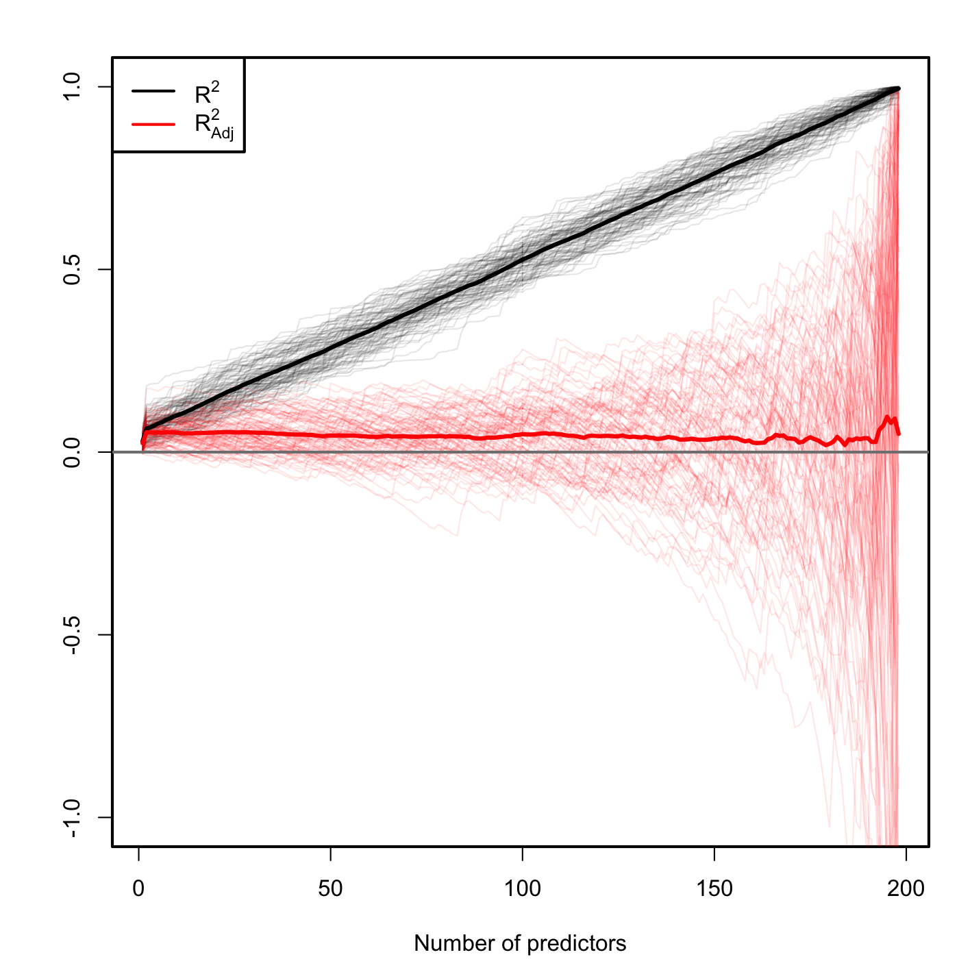
Figure 2.1: Comparison of \(R^2\) and \(R^2_{\text{adj}}\) for \(n=200\) and \(p\) ranging from \(1\) to \(198\). \(M=100\) datasets were simulated with only the first two predictors being significant. The thicker curves are the mean of each color’s curves.

Figure 2.1 contains the results of an experiment where 100 datasets were simulated with only the first two predictors being significant. As you can see \(R^2\) increases linearly with the number of predictors considered, although only the first two ones were important! On the contrary, \(R^2_\text{adj}\) only increases in the first two variables and then is flat on average, but it has a huge variability when \(p\) approaches \(n-2\). The experiment evidences that \(R^2_\text{adj}\) is more adequate than the \(R^2\) for evaluating the fit of a multiple linear regression.

Have a look at the residuals or error terms

What is often ignored are error terms or so-called residuals. They often tell you more than what you might think. The residuals are the difference between your predicted values and the actual values. Their benefit is that they can show both the magnitude as well as the direction of the errors.

Let’s have a look at an example:

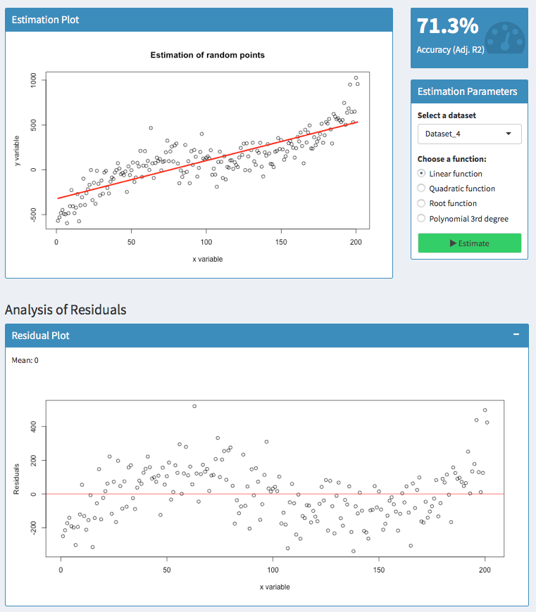
Here, we try to predict a polynomial dataset with a linear function. Analyzing the residuals shows that there are areas where the model has an upward or downward bias.

For 50 < x < 100, the residuals are above zero. So in this area, the actual values have been higher than the predicted values — our model has a downward bias.

For 100 < x < 150, however, the residuals are below zero. Thus, the actual values have been lower than the predicted values — the model has an upward bias.

It is always good to know, whether your model suggests too high or too low values. But you usually do not want to have patterns like this.

The residuals should be zero on average (as indicated by the mean) and they should be equally distributed. Predicting the same dataset with a polynomial function of 3 degrees suggests a much better fit:

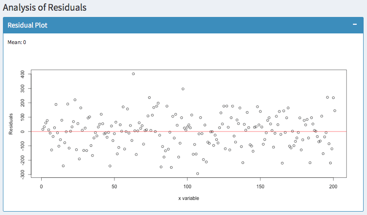
In addition, you can observe whether the variance of your errors increases. In statistics, this is called Heteroscedasticity. You can fix this easily with robust standard errors. Otherwise, your hypothesis tests are likely to be wrong.

Histogram of residuals

Finally, the histogram summarizes the magnitude of your error terms. It provides information about the bandwidth of errors and indicates how often which errors occurred.

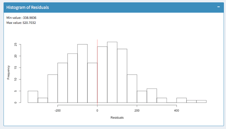
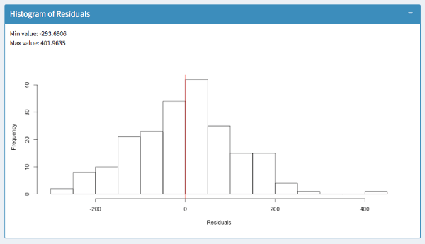
The above screenshots show two models for the same dataset. In the first histogram, errors occur within a range of -338 and 520. In the second histogram, errors occur within -293 and 401. So the outliers are much lower. Furthermore, most errors in the model of the second histogram are closer to zero. So we would favor the second model.

◼