6 Principal Components Analysis
6.1 Introduction
The central idea of principal component analysis (PCA) is to reduce the dimensionality of a data set consisting of a large number of interrelated variables, while retaining as much as possible of the variation present in the data set. This is achieved by transforming to a new set of variables, the principal components (PCs), which are uncorrelated, and which are ordered so that the first few retain most of the variation present in all of the original variables.
Suppose that we wish to visualize \(n\) observations with measurements on a set of \(p\) features, \(X_1,X_2,\ldots,X_p\), as part of an exploratory data analysis. We could do this by examining two-dimensional scatterplots of the data, each of which contains the \(n\) observations’ measurements on two of the features. However, there are \(C_p^2 = p(p−1)/2\) such scatterplots. For example, with \(p =10\) there are 45 plots! If \(p\) is large, then it will certainly not be possible to look at all of them; moreover, most likely none of them will be informative since they each contain just a small fraction of the total information present in the data set. Clearly, a better method is required to visualize the \(n\) observations when \(p\) is large. In particular, we would like to find a low-dimensional representation of the data that captures as much of the information as possible. PCA provides a tool to do just this.
PCA finds a low-dimensional representation of a data set that contains as much as possible of the variation. The idea is that each of the \(n\) observations lives in \(p\)-dimensional space, but not all of these dimensions are equally interesting. PCA seeks a small number of dimensions that are as interesting as possible, where the concept of interesting is measured by the amount that the observations vary along each dimension. Each of the dimensions found by PCA is a linear combination of the \(p\) features. We now explain the manner in which these dimensions, or principal components, are found.
6.2 Principal Components
Notations and Procedure
Suppose that we have a random vector of the features \(X\).
\[ \textbf{X} = \left(\begin{array}{c} X_1\\ X_2\\ \vdots \\X_p\end{array}\right) \]
with population variance-covariance matrix
\[ \text{var}(\textbf{X}) = \Sigma = \left(\begin{array}{cccc}\sigma^2_1 & \sigma_{12} & \dots &\sigma_{1p}\\ \sigma_{21} & \sigma^2_2 & \dots &\sigma_{2p}\\ \vdots & \vdots & \ddots & \vdots \\ \sigma_{p1} & \sigma_{p2} & \dots & \sigma^2_p\end{array}\right) \]
Consider the linear combinations
\[ \begin{array}{lll} Y_1 & = & a_{11}X_1 + a_{12}X_2 + \dots + a_{1p}X_p \\ Y_2 & = & a_{21}X_1 + a_{22}X_2 + \dots + a_{2p}X_p \\ & & \vdots \\ Y_p & = & a_{p1}X_1 + a_{p2}X_2 + \dots +a_{pp}X_p \end{array} \]
Note that \(Y_i\) is a function of our random data, and so is also random. Therefore it has a population variance
\[ \text{var}(Y_i) = \sum_{k=1}^{p} \sum_{l=1}^{p} a_{ik} a_{il} \sigma_{kl} = \mathbf{a}^T_i \Sigma \mathbf{a}_i \]
Moreover, \(Y_i\) and \(Y_j\) will have a population covariance
\[ \text{cov}(Y_i, Y_j) = \sum_{k=1}^{p} \sum_{l=1}^{p} a_{ik}a_{jl}\sigma_{kl} = \mathbf{a}^T_i\Sigma\mathbf{a}_j \]
and a correlation
\[ \text{cor}(Y_i, Y_j) = \frac{\text{cov}(Y_i, Y_j)}{\sigma^2_i \sigma^2_j}\]
Here the coefficients \(a_{ij}\) are collected into the vector
\[ \mathbf{a}_i = \left(\begin{array}{c} a_{i1}\\ a_{i2}\\ \vdots \\ a_{ip}\end{array}\right) \]
The coefficients \(a_{ij}\) are also called loadings of the principal component \(i\) and \(\mathbf{a}_i\) is a principal component loading vector.
- The total variation of \(X\) is the trace of the variance-covariance matrix \(\Sigma\).
- The trace of \(\Sigma\) is the sum of the variances of the individual variables.
- \(trace(\Sigma) \, = \, \sigma^2_1 + \sigma^2_2 + \dots +\sigma^2_p\)
First Principal Component (\(\text{PC}_1\)): \(Y_1\)
The first principal component is the normalized linear combination of the features \(X_1,X_2,\ldots,X_p\) that has maximum variance (among all linear combinations), so it accounts for as much variation in the data as possible.
Specifically we will define coefficients \(a_{11},a_{12},\ldots,a_{1p}\) for that component in such a way that its variance is maximized, subject to the constraint that the sum of the squared coefficients is equal to one (that is what we mean by normalized). This constraint is required so that a unique answer may be obtained.
More formally, select \(a_{11},a_{12},\ldots,a_{1p}\) that maximizes
\[ \text{var}(Y_1) = \mathbf{a}^T_1\Sigma\mathbf{a}_1 = \sum_{k=1}^{p}\sum_{l=1}^{p}a_{1k}a_{1l}\sigma_{kl} \]
subject to the constraint that
\[ \sum_{j=1}^{p}a^2_{1j} = \mathbf{a}^T_1\mathbf{a}_1 = 1 \]
Second Principal Component (\(\text{PC}_2\)): \(Y_2\)
The second principal component is the linear combination of the features \(X_1,X_2,\ldots,X_p\) that accounts for as much of the remaining variation as possible, with the constraint that the correlation between the first and second component is 0. So the second principal component has maximal variance out of all linear combinations that are uncorrelated with \(Y_1\).
To compute the coefficients of the second principal component, we select \(a_{21},a_{22},\ldots,a_{2p}\) that maximizes the variance of this new component
\[\text{var}(Y_2) = \sum_{k=1}^{p}\sum_{l=1}^{p}a_{2k}a_{2l}\sigma_{kl} = \mathbf{a}^T_2\Sigma\mathbf{a}_2 \]
subject to:
The constraint that the sums of squared coefficients add up to one, \(\sum_{j=1}^{p}a^2_{2j} = \mathbf{a}^T_2\mathbf{a}_2 = 1\).
Along with the additional constraint that these two components will be uncorrelated with one another:
\[ \text{cov}(Y_1, Y_2) = \mathbf{a}^T_1\Sigma\mathbf{a}_2 = \sum_{k=1}^{p}\sum_{l=1}^{p}a_{1k}a_{2l}\sigma_{kl} = 0 \]
All subsequent principal components have this same property: they are linear combinations that account for as much of the remaining variation as possible and they are not correlated with the other principal components.
We will do this in the same way with each additional component. For instance:
\(i^{th}\) Principal Component (\(\text{PC}_i\)): \(Y_i\)
We select \(a_{i1},a_{i2},\ldots,a_{ip}\) that maximizes
\[ \text{var}(Y_i) = \sum_{k=1}^{p}\sum_{l=1}^{p}a_{ik}a_{il}\sigma_{kl} = \mathbf{a}^T_i\Sigma\mathbf{a}_i \]
subject to the constraint that the sums of squared coefficients add up to one, along with the additional constraint that this new component will be uncorrelated with all the previously defined components:
\[ \sum_{j=1}^{p}a^2_{ij} \mathbf{a}^T_i\mathbf{a}_i = \mathbf{a}^T_i\mathbf{a}_i = 1\]
\[ \text{cov}(Y_1, Y_i) = \sum_{k=1}^{p}\sum_{l=1}^{p}a_{1k}a_{il}\sigma_{kl} = \mathbf{a}^T_1\Sigma\mathbf{a}_i = 0 \]
\[\text{cov}(Y_2, Y_i) = \sum_{k=1}^{p}\sum_{l=1}^{p}a_{2k}a_{il}\sigma_{kl} = \mathbf{a}^T_2\Sigma\mathbf{a}_i = 0\] \[\vdots\] \[\text{cov}(Y_{i-1}, Y_i) = \sum_{k=1}^{p}\sum_{l=1}^{p}a_{i-1,k}a_{il}\sigma_{kl} = \mathbf{a}^T_{i-1}\Sigma\mathbf{a}_i = 0\]
Therefore all principal components are uncorrelated with one another.
6.3 How do we find the coefficients?
How do we find the coefficients \(a_{ij}\) for a principal component? The solution involves the eigenvalues and eigenvectors of the variance-covariance matrix \(\Sigma\).
Let \(\lambda_1,\ldots,\lambda_p\) denote the eigenvalues of the variance-covariance matrix \(\Sigma\). These are ordered so that \(\lambda_1\) has the largest eigenvalue and \(\lambda_p\) is the smallest.
\[ \lambda_1 \ge \lambda_2 \ge \dots \ge \lambda_p \]
We are also going to let the vectors \(\mathbf{a}_1, \ldots,\mathbf{a}_p\) denote the corresponding eigenvectors.
It turns out that the elements for these eigenvectors will be the coefficients of the principal components.
The elements for the eigenvectors of \(\Sigma\) are the coefficients of the principal components.
The variance for the \(i\)th principal component is equal to the \(i\)th eigenvalue.
\[ \textbf{var}(Y_i) = \text{var}(a_{i1}X_1 + a_{i2}X_2 + \dots a_{ip}X_p) = \lambda_i \]
Moreover, the principal components are uncorrelated with one another.
\[\text{cov}(Y_i, Y_j) = 0\]
The variance-covariance matrix may be written as a function of the eigenvalues and their corresponding eigenvectors. In fact, the variance-covariance matrix can be written as the sum over the \(p\) eigenvalues, multiplied by the product of the corresponding eigenvector times its transpose as shown in the following expression
\[ \Sigma = \sum_{i=1}^{p}\lambda_i \mathbf{a}_i \mathbf{a}_i^T \]
If \(\lambda_{k+1}, \lambda_{k+2}, \dots , \lambda_{p}\) are small, we might approximate \(\Sigma\) by
\[ \Sigma \cong \sum_{i=1}^{k}\lambda_i \mathbf{a}_i\mathbf{a}_i^T \]
Earlier in the chapter we defined the total variation of \(X\) as the trace of the variance-covariance matrix. This is also equal to the sum of the eigenvalues as shown below:
\[ \begin{array}{lll}trace(\Sigma) & = & \sigma^2_1 + \sigma^2_2 + \dots +\sigma^2_p \\ & = & \lambda_1 + \lambda_2 + \dots + \lambda_p\end{array} \]
This will give us an interpretation of the components in terms of the amount of the full variation explained by each component. The proportion of variation explained by the \(i\)th principal component is then going to be defined to be the eigenvalue for that component divided by the sum of the eigenvalues. In other words, the \(i\)th principal component explains the following proportion of the total variation:
\[ \frac{\lambda_i}{\lambda_1 + \lambda_2 + \dots + \lambda_p} \]
A related quantity is the proportion of variation explained by the first \(k\) principal component. This would be the sum of the first \(k\) eigenvalues divided by its total variation.
\[ \frac{\lambda_1 + \lambda_2 + \dots + \lambda_k}{\lambda_1 + \lambda_2 + \dots + \lambda_p} \]
In practice, these proportions are often expressed as percentages.
Naturally, if the proportion of variation explained by the first \(k\) principal components is large, then not much information is lost by considering only the first \(k\) principal components.
Why It May Be Possible to Reduce Dimensions
When we have correlations (multicollinarity) between the features, the data may more or less fall on a line or plane in a lower number of dimensions. For instance, imagine a plot of two features that have a nearly perfect correlation. The data points will fall close to a straight line. That line could be used as a new (one-dimensional) axis to represent the variation among data points.
All of this is defined in terms of the population variance-covariance matrix \(\Sigma\) which is unknown. However, we may estimate \(\Sigma\) by the sample variance-covariance matrix which is given in the standard formula here:
\[ \textbf{S} = \frac{1}{n-1} \sum_{i=1}^{n}(\mathbf{X}_i-\bar{\textbf{x}})(\mathbf{X}_i-\bar{\textbf{x}})^T \]
Procedure
Compute the eigenvalues \(\hat{\lambda}_1, \hat{\lambda}_2, \dots, \hat{\lambda}_p\) of the sample variance-covariance matrix \(\textbf{S}\), and the corresponding eigenvectors \(\hat{\mathbf{a}}_1, \hat{\mathbf{a}}_2, \dots, \hat{\mathbf{a}}_p\).
Then we will define our estimated principal components using the eigenvectors as our coefficients:
\[ \begin{array}{lll} \hat{Y}_1 & = & \hat{a}_{11}X_1 + \hat{a}_{12}X_2 + \dots + \hat{a}_{1p}X_p \\ \hat{Y}_2 & = & \hat{a}_{21}X_1 + \hat{a}_{22}X_2 + \dots + \hat{a}_{2p}X_p \\&&\vdots\\ \hat{Y}_p & = & \hat{a}_{p1}X_1 + \hat{a}_{p2}X_2 + \dots + \hat{a}_{pp}X_p \\ \end{array} \]
Generally, we only retain the first \(k\) principal component. There are a number of criteria that may be used to decide how many components should be retained:
To obtain the simplest possible interpretation, we want \(k\) to be as small as possible. If we can explain most of the variation just by two principal components then this would give us a much simpler description of the data.
Retain the first \(k\) components which explain a “large” proportion of the total variation, say \(70-80\%\).
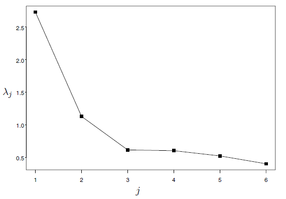
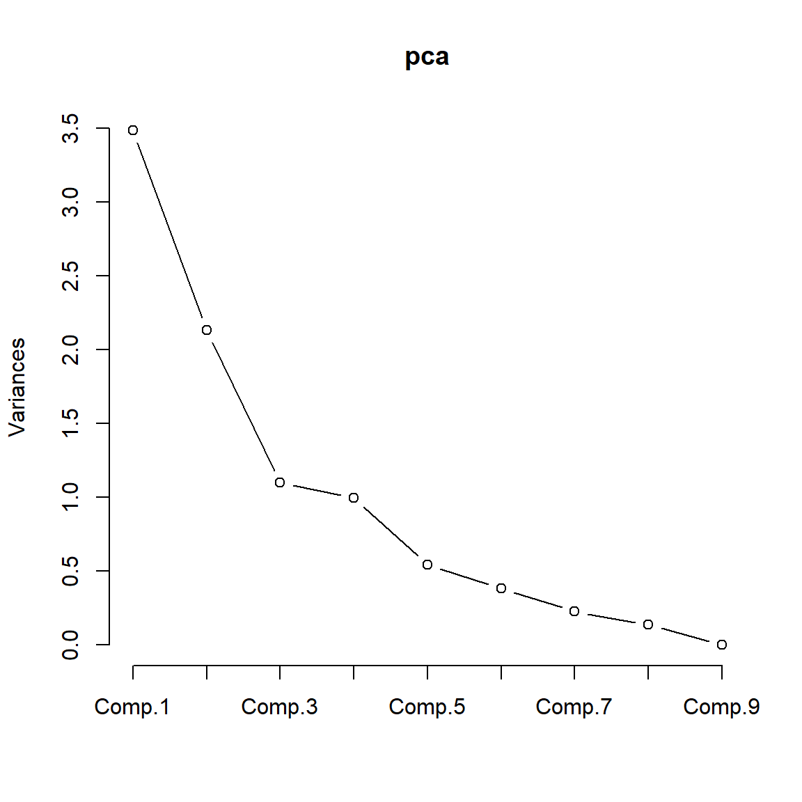
Examine a scree plot. This is a plot of the eigenvalues versus the component number. The idea is to look for the “elbow” which corresponds to the point after which the eigenvalues decrease more slowly. Adding components after this point explains relatively little more of the variance. See the next figure for an example of a scree plot.
6.4 Standardization of the features
If we use the raw data, the principal component analysis will tend to give more emphasis to the variables that have higher variances than to those variables that have very low variances.
In effect the results of the analysis will depend on what units of measurement are used to measure each variable. That would imply that a principal component analysis should only be used with the raw data if all variables have the same units of measure. And even in this case, only if you wish to give those variables which have higher variances more weight in the analysis.
- The results of principal component analysis depend on the scales at which the variables are measured.
- Variables with the highest sample variances will tend to be emphasized in the first few principal components.
- Principal component analysis using the covariance function should only be considered if all of the variables have the same units of measurement.
If the variables either have different units of measurement, or if we wish each variable to receive equal weight in the analysis, then the variables should be standardized (scaled) before a principal components analysis is carried out. Standardize the variables by subtracting its mean from that variable and dividing it by its standard deviation:
\[Z_{ij} = \frac{X_{ij}-\bar{x}_j}{\sigma_j}\]
where
- \(X_{ij}\) = Data for variable \(j\) in sample unit \(i\)
- \(\bar{x}_j\) = Sample mean for variable \(j\)
- \(\sigma_j\) = Sample standard deviation for variable \(j\)
Note: \(Z_j\) has mean = 0 and variance = 1.
The variance-covariance matrix of the standardized data is equal to the correlation matrix for the unstandardized data. Therefore, principal component analysis using the standardized data is equivalent to principal component analysis using the correlation matrix. Remark: You are going to prove it in the practical work session.
6.5 Projection of the data
Scores
Using the coefficients (loadings) of every principal component, we can project the observations on the axis of the principal component, those projections are called scores. For example, the scores of the first principal component are
\[ \forall 1 \le i \le n \quad \hat{Y}_1^i = \hat{a}_{11}X_1^i + \hat{a}_{12}X_2^i + \dots + \hat{a}_{1p}X_p^i \]
(\(X_1^i\) is the value of feature \(1\) for the observation \(i\))
This can be written for all observations and all the principal components using the matrix formulation
\[ \mathbf{\hat{Y}} = \mathbf{\hat{A}} X\]
where \(\mathbf{\hat{A}}\) is the matrix of the coefficients \(\hat{a}_{ij}\).
Visualization
Once we have computed the principal components, we can plot them against each other in order to produce low-dimensional views of the data.
We can plot the score vector \(Y_1\) against \(Y_2\), \(Y_1\) against \(Y_3\), \(Y_2\) against \(Y_3\), and so forth. Geometrically, this amounts to projecting the original data down onto the subspace spanned by \(\mathbf{a}_1\), \(\mathbf{a}_2\), and \(\mathbf{a}_3\), and plotting the projected points.
To interpret the results obtained by PCA, we plot on the same figure both the principal component scores and the loading vectors. This figure is called a biplot. An example is given later in this chapter.
6.6 Case study
Employement in European countries in the late 70s
The purpose of this case study is to reveal the structure of the job market and economy in different developed countries. The final aim is to have a meaningful and rigorous plot that is able to show the most important features of the countries in a concise form.
The dataset eurojob contains the data employed in this case study. It contains the percentage of workforce employed in 1979 in 9 industries for 26 European countries. The industries measured are:
- Agriculture (
Agr) - Mining (
Min) - Manufacturing (
Man) - Power supply industries
(Pow) - Construction (
Con) - Service industries (
Ser) - Finance (
Fin) - Social and personal services (
Soc) - Transport and communications (
Tra)
If the dataset is imported into and the case names are set as Country (important in order to have only numerical variables), then the data should look like this:
| Country | Agr | Min | Man | Pow | Con | Ser | Fin | Soc | Tra |
|---|---|---|---|---|---|---|---|---|---|
| Belgium | 3.3 | 0.9 | 27.6 | 0.9 | 8.2 | 19.1 | 6.2 | 26.6 | 7.2 |
| Denmark | 9.2 | 0.1 | 21.8 | 0.6 | 8.3 | 14.6 | 6.5 | 32.2 | 7.1 |
| France | 10.8 | 0.8 | 27.5 | 0.9 | 8.9 | 16.8 | 6.0 | 22.6 | 5.7 |
| WGerm | 6.7 | 1.3 | 35.8 | 0.9 | 7.3 | 14.4 | 5.0 | 22.3 | 6.1 |
| Ireland | 23.2 | 1.0 | 20.7 | 1.3 | 7.5 | 16.8 | 2.8 | 20.8 | 6.1 |
| Italy | 15.9 | 0.6 | 27.6 | 0.5 | 10.0 | 18.1 | 1.6 | 20.1 | 5.7 |
| Luxem | 7.7 | 3.1 | 30.8 | 0.8 | 9.2 | 18.5 | 4.6 | 19.2 | 6.2 |
| Nether | 6.3 | 0.1 | 22.5 | 1.0 | 9.9 | 18.0 | 6.8 | 28.5 | 6.8 |
| UK | 2.7 | 1.4 | 30.2 | 1.4 | 6.9 | 16.9 | 5.7 | 28.3 | 6.4 |
| Austria | 12.7 | 1.1 | 30.2 | 1.4 | 9.0 | 16.8 | 4.9 | 16.8 | 7.0 |
| Finland | 13.0 | 0.4 | 25.9 | 1.3 | 7.4 | 14.7 | 5.5 | 24.3 | 7.6 |
| Greece | 41.4 | 0.6 | 17.6 | 0.6 | 8.1 | 11.5 | 2.4 | 11.0 | 6.7 |
| Norway | 9.0 | 0.5 | 22.4 | 0.8 | 8.6 | 16.9 | 4.7 | 27.6 | 9.4 |
| Portugal | 27.8 | 0.3 | 24.5 | 0.6 | 8.4 | 13.3 | 2.7 | 16.7 | 5.7 |
| Spain | 22.9 | 0.8 | 28.5 | 0.7 | 11.5 | 9.7 | 8.5 | 11.8 | 5.5 |
| Sweden | 6.1 | 0.4 | 25.9 | 0.8 | 7.2 | 14.4 | 6.0 | 32.4 | 6.8 |
| Switz | 7.7 | 0.2 | 37.8 | 0.8 | 9.5 | 17.5 | 5.3 | 15.4 | 5.7 |
| Turkey | 66.8 | 0.7 | 7.9 | 0.1 | 2.8 | 5.2 | 1.1 | 11.9 | 3.2 |
| Bulgaria | 23.6 | 1.9 | 32.3 | 0.6 | 7.9 | 8.0 | 0.7 | 18.2 | 6.7 |
| Czech | 16.5 | 2.9 | 35.5 | 1.2 | 8.7 | 9.2 | 0.9 | 17.9 | 7.0 |
| EGerm | 4.2 | 2.9 | 41.2 | 1.3 | 7.6 | 11.2 | 1.2 | 22.1 | 8.4 |
| Hungary | 21.7 | 3.1 | 29.6 | 1.9 | 8.2 | 9.4 | 0.9 | 17.2 | 8.0 |
| Poland | 31.1 | 2.5 | 25.7 | 0.9 | 8.4 | 7.5 | 0.9 | 16.1 | 6.9 |
| Romania | 34.7 | 2.1 | 30.1 | 0.6 | 8.7 | 5.9 | 1.3 | 11.7 | 5.0 |
| USSR | 23.7 | 1.4 | 25.8 | 0.6 | 9.2 | 6.1 | 0.5 | 23.6 | 9.3 |
| Yugoslavia | 48.7 | 1.5 | 16.8 | 1.1 | 4.9 | 6.4 | 11.3 | 5.3 | 4.0 |
Note: To set the case names as Country, we do
So far, we know how to compute summaries for each variable, and how to quantify and visualize relations between variables with the correlation matrix and the scatterplot matrix. But even for a moderate number of variables like this, their results are hard to process.
# Summary of the data - marginal
summary(eurojob)
#ans> Agr Min Man Pow
#ans> Min. : 2.7 Min. :0.100 Min. : 7.9 Min. :0.100
#ans> 1st Qu.: 7.7 1st Qu.:0.525 1st Qu.:23.0 1st Qu.:0.600
#ans> Median :14.4 Median :0.950 Median :27.6 Median :0.850
#ans> Mean :19.1 Mean :1.254 Mean :27.0 Mean :0.908
#ans> 3rd Qu.:23.7 3rd Qu.:1.800 3rd Qu.:30.2 3rd Qu.:1.175
#ans> Max. :66.8 Max. :3.100 Max. :41.2 Max. :1.900
#ans> Con Ser Fin Soc
#ans> Min. : 2.80 Min. : 5.20 Min. : 0.50 Min. : 5.3
#ans> 1st Qu.: 7.53 1st Qu.: 9.25 1st Qu.: 1.23 1st Qu.:16.2
#ans> Median : 8.35 Median :14.40 Median : 4.65 Median :19.6
#ans> Mean : 8.17 Mean :12.96 Mean : 4.00 Mean :20.0
#ans> 3rd Qu.: 8.97 3rd Qu.:16.88 3rd Qu.: 5.92 3rd Qu.:24.1
#ans> Max. :11.50 Max. :19.10 Max. :11.30 Max. :32.4
#ans> Tra
#ans> Min. :3.20
#ans> 1st Qu.:5.70
#ans> Median :6.70
#ans> Mean :6.55
#ans> 3rd Qu.:7.08
#ans> Max. :9.40
# Correlation matrix
cor(eurojob)
#ans> Agr Min Man Pow Con Ser Fin Soc Tra
#ans> Agr 1.0000 0.0358 -0.671 -0.4001 -0.5383 -0.737 -0.2198 -0.747 -0.565
#ans> Min 0.0358 1.0000 0.445 0.4055 -0.0256 -0.397 -0.4427 -0.281 0.157
#ans> Man -0.6711 0.4452 1.000 0.3853 0.4945 0.204 -0.1558 0.154 0.351
#ans> Pow -0.4001 0.4055 0.385 1.0000 0.0599 0.202 0.1099 0.132 0.375
#ans> Con -0.5383 -0.0256 0.494 0.0599 1.0000 0.356 0.0163 0.158 0.388
#ans> Ser -0.7370 -0.3966 0.204 0.2019 0.3560 1.000 0.3656 0.572 0.188
#ans> Fin -0.2198 -0.4427 -0.156 0.1099 0.0163 0.366 1.0000 0.108 -0.246
#ans> Soc -0.7468 -0.2810 0.154 0.1324 0.1582 0.572 0.1076 1.000 0.568
#ans> Tra -0.5649 0.1566 0.351 0.3752 0.3877 0.188 -0.2459 0.568 1.000
# Scatterplot matrix
require(car)
scatterplotMatrix(eurojob, regLine = list(method=lm, lty=1, lwd=2, col="green"), smooth = FALSE,
ellipse = FALSE, plot.points = T, col="black",
diagonal = TRUE)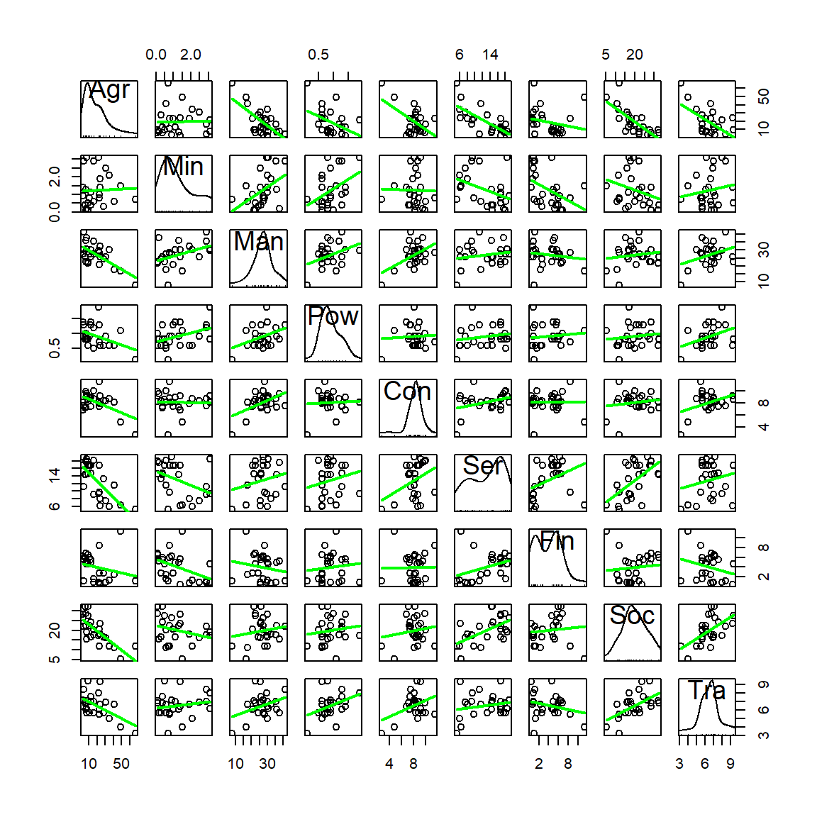 We definitely need a way of visualizing and quantifying the relations between variables for a moderate to large amount of variables. PCA will be a handy way. Recall what PCA does:
- Takes the data for the variables \(X_1,\ldots,X_p\).
- Using this data, looks for new variables \(\text{PC}_1,\ldots \text{PC}_p\) such that:
- \(\text{PC}_j\) is a linear combination of \(X_1,\ldots,X_k\), \(1\leq j\leq p\). This is, \(\text{PC}_j=a_{1j}X_1+a_{2j}X_2+\ldots+a_{pj}X_p\).
- \(\text{PC}_1,\ldots \text{PC}_p\) are sorted decreasingly in terms of variance. Hence \(\text{PC}_j\) has more variance than \(\text{PC}_{j+1}\), \(1\leq j\leq p-1\),
- \(\text{PC}_{j_1}\) and \(\text{PC}_{j_2}\) are uncorrelated, for \(j_1\neq j_2\).
- \(\text{PC}_1,\ldots \text{PC}_p\) have the same information, measured in terms of total variance, as \(X_1,\ldots,X_p\).
- Produces three key objects:
- Variances of the PCs. They are sorted decreasingly and give an idea of which PCs are contain most of the information of the data (the ones with more variance).
- Weights of the variables in the PCs. They give the interpretation of the PCs in terms of the original variables, as they are the coefficients of the linear combination. The weights of the variables \(X_1,\ldots,X_p\) on the PC\(_j\), \(a_{1j},\ldots,a_{pj}\), are normalized: \(a_{1j}^2+\ldots+a_{pj}^2=1\), \(j=1,\ldots,p\). In , they are called
loadings. - Scores of the data in the PCs: this is the data with \(\text{PC}_1,\ldots \text{PC}_p\) variables instead of \(X_1,\ldots,X_p\). The scores are uncorrelated. Useful for knowing which PCs have more effect on a certain observation.
Hence, PCA rearranges our variables in an information-equivalent, but more convenient, layout where the variables are sorted according to the ammount of information they are able to explain. From this position, the next step is clear: stick only with a limited number of PCs such that they explain most of the information (e.g., 70% of the total variance) and do dimension reduction. The effectiveness of PCA in practice varies from the structure present in the dataset. For example, in the case of highly dependent data, it could explain more than the 90% of variability of a dataset with tens of variables with just two PCs.
Let’s see how to compute a full PCA in .
# The main function - use cor = TRUE to avoid scale distortions
pca <- princomp(eurojob, cor = TRUE)

# What is inside?
str(pca)
#ans> List of 7
#ans>  $ sdev    : Named num [1:9] 1.867 1.46 1.048 0.997 0.737 ...
#ans>   ..- attr(*, "names")= chr [1:9] "Comp.1" "Comp.2" "Comp.3" "Comp.4" ...
#ans>  $ loadings: 'loadings' num [1:9, 1:9] 0.52379 0.00132 -0.3475 -0.25572 -0.32518 ...
#ans>   ..- attr(*, "dimnames")=List of 2
#ans>   .. ..$ : chr [1:9] "Agr" "Min" "Man" "Pow" ...
#ans>   .. ..$ : chr [1:9] "Comp.1" "Comp.2" "Comp.3" "Comp.4" ...
#ans>  $ center  : Named num [1:9] 19.131 1.254 27.008 0.908 8.165 ...
#ans>   ..- attr(*, "names")= chr [1:9] "Agr" "Min" "Man" "Pow" ...
#ans>  $ scale   : Named num [1:9] 15.245 0.951 6.872 0.369 1.614 ...
#ans>   ..- attr(*, "names")= chr [1:9] "Agr" "Min" "Man" "Pow" ...
#ans>  $ n.obs   : int 26
#ans>  $ scores  : num [1:26, 1:9] -1.71 -0.953 -0.755 -0.853 0.104 ...
#ans>   ..- attr(*, "dimnames")=List of 2
#ans>   .. ..$ : chr [1:26] "Belgium" "Denmark" "France" "WGerm" ...
#ans>   .. ..$ : chr [1:9] "Comp.1" "Comp.2" "Comp.3" "Comp.4" ...
#ans>  $ call    : language princomp(x = eurojob, cor = TRUE)
#ans>  - attr(*, "class")= chr "princomp"

# The standard deviation of each PC
pca$sdev
#ans>  Comp.1  Comp.2  Comp.3  Comp.4  Comp.5  Comp.6  Comp.7  Comp.8  Comp.9
#ans> 1.86739 1.45951 1.04831 0.99724 0.73703 0.61922 0.47514 0.36985 0.00675

# Weights: the expression of the original variables in the PCs
# E.g. Agr = -0.524 * PC1 + 0.213 * PC5 - 0.152 * PC6 + 0.806 * PC9
# And also: PC1 = -0.524 * Agr + 0.347 * Man + 0256 * Pow + 0.325 * Con + ...
# (Because the matrix is orthogonal, so the transpose is the inverse)
pca$loadings
#ans>
#ans> Loadings:
#ans>     Comp.1 Comp.2 Comp.3 Comp.4 Comp.5 Comp.6 Comp.7 Comp.8 Comp.9
#ans> Agr  0.524                       0.213  0.153                0.806
#ans> Min         0.618 -0.201        -0.164 -0.101 -0.726
#ans> Man -0.347  0.355 -0.150 -0.346 -0.385 -0.288  0.479  0.126  0.366
#ans> Pow -0.256  0.261 -0.561  0.393  0.295  0.357  0.256 -0.341
#ans> Con -0.325         0.153 -0.668  0.472  0.130 -0.221 -0.356
#ans> Ser -0.379 -0.350 -0.115        -0.284  0.615 -0.229  0.388  0.238
#ans> Fin        -0.454 -0.587         0.280 -0.526 -0.187  0.174  0.145
#ans> Soc -0.387 -0.222  0.312  0.412 -0.220 -0.263 -0.191 -0.506  0.351
#ans> Tra -0.367  0.203  0.375  0.314  0.513 -0.124         0.545
#ans>
#ans>                Comp.1 Comp.2 Comp.3 Comp.4 Comp.5 Comp.6 Comp.7 Comp.8
#ans> SS loadings     1.000  1.000  1.000  1.000  1.000  1.000  1.000  1.000
#ans> Proportion Var  0.111  0.111  0.111  0.111  0.111  0.111  0.111  0.111
#ans> Cumulative Var  0.111  0.222  0.333  0.444  0.556  0.667  0.778  0.889
#ans>                Comp.9
#ans> SS loadings     1.000
#ans> Proportion Var  0.111
#ans> Cumulative Var  1.000

# Scores of the data on the PCs: how is the data reexpressed into PCs
head(pca$scores, 10)
#ans>         Comp.1  Comp.2  Comp.3  Comp.4  Comp.5  Comp.6  Comp.7 Comp.8
#ans> Belgium -1.710 -1.2218 -0.1148  0.3395 -0.3245 -0.0473 -0.3401  0.403
#ans> Denmark -0.953 -2.1278  0.9507  0.5939  0.1027 -0.8273 -0.3029 -0.352
#ans> France  -0.755 -1.1212 -0.4980 -0.5003 -0.2997  0.1158 -0.1855 -0.266
#ans> WGerm   -0.853 -0.0114 -0.5795 -0.1105 -1.1652 -0.6181  0.4446  0.194
#ans> Ireland  0.104 -0.4140 -0.3840  0.9267  0.0152  1.4242 -0.0370 -0.334
#ans> Italy   -0.375 -0.7695  1.0606 -1.4772 -0.6452  1.0021 -0.1418 -0.130
#ans> Luxem   -1.059  0.7558 -0.6515 -0.8352 -0.8659  0.2188 -1.6942  0.547
#ans> Nether  -1.688 -2.0048  0.0637 -0.0235  0.6352  0.2120 -0.3034 -0.591
#ans> UK      -1.630 -0.3731 -1.1409  1.2669 -0.8129 -0.0361  0.0413 -0.349
#ans> Austria -1.176  0.1431 -1.0434 -0.1577  0.5210  0.8019  0.4150  0.215
#ans>            Comp.9
#ans> Belgium -0.001090
#ans> Denmark  0.015619
#ans> France  -0.000507
#ans> WGerm   -0.006539
#ans> Ireland  0.010879
#ans> Italy    0.005602
#ans> Luxem    0.003453
#ans> Nether  -0.010931
#ans> UK      -0.005478
#ans> Austria -0.002816

# Scatterplot matrix of the scores - See how they are uncorrelated!
scatterplotMatrix(pca$scores, regLine = list(method=lm, lty=1, lwd=2, col="green"), smooth = FALSE,
                  ellipse = FALSE, plot.points = T, col="black",
                  diagonal = TRUE)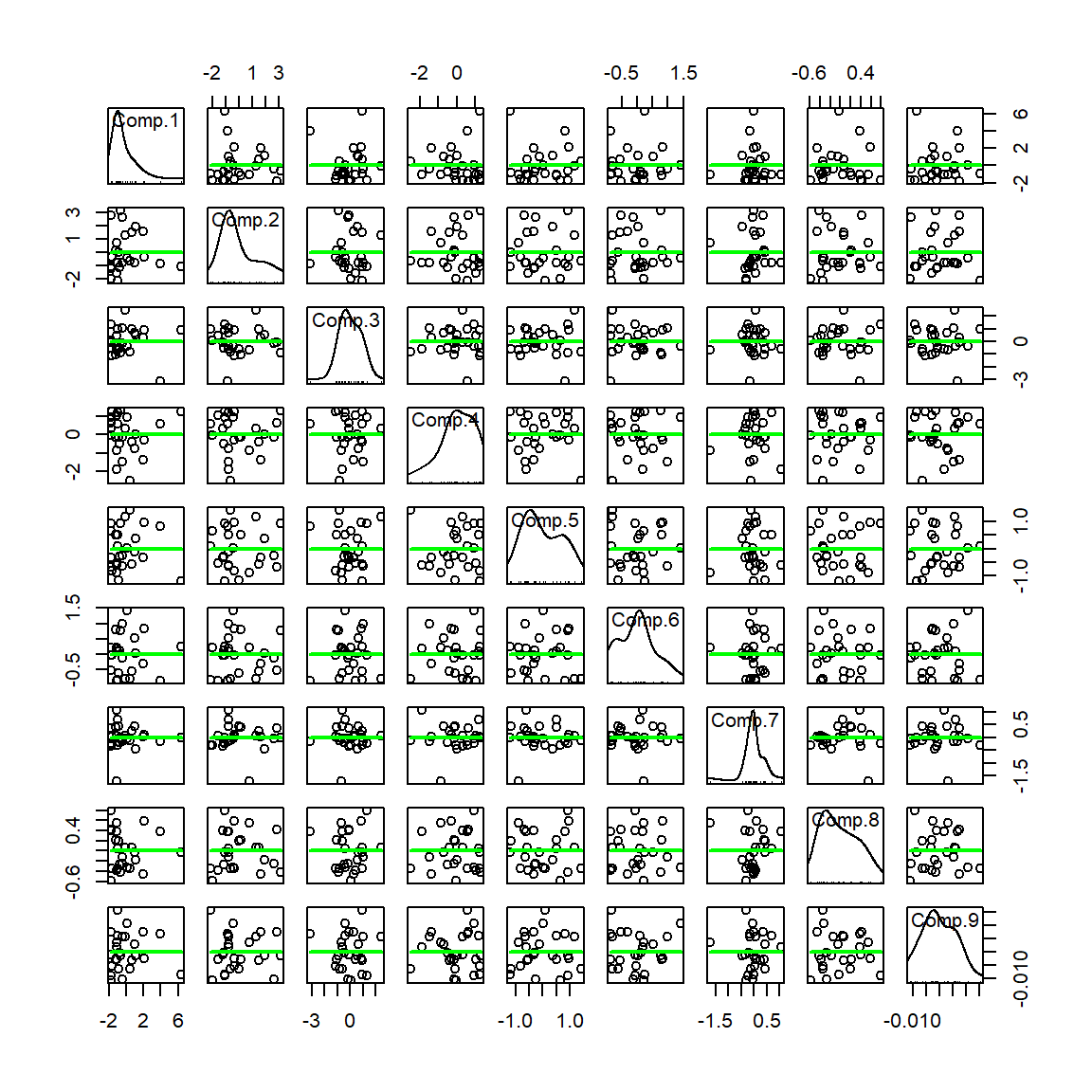
PCA produces uncorrelated variables from the original set \(X_1,\ldots,X_p\). This implies that:
- The PCs are uncorrelated, but not independent (uncorrelated does not imply independent).
- An uncorrelated or independent variable in \(X_1,\ldots,X_p\) will get a PC only associated to it. In the extreme case where all the \(X_1,\ldots,X_p\) are uncorrelated, these coincide with the PCs (up to sign flips).
# Means of the variables - before PCA the variables are centered
pca$center
#ans>    Agr    Min    Man    Pow    Con    Ser    Fin    Soc    Tra
#ans> 19.131  1.254 27.008  0.908  8.165 12.958  4.000 20.023  6.546

# Rescalation done to each variable
# - if cor = FALSE (default), a vector of ones
# - if cor = TRUE, a vector with the standard deviations of the variables
pca$scale
#ans>    Agr    Min    Man    Pow    Con    Ser    Fin    Soc    Tra
#ans> 15.245  0.951  6.872  0.369  1.614  4.486  2.752  6.697  1.364

# Summary of the importance of components - the third row is key
summary(pca)
#ans> Importance of components:
#ans>                        Comp.1 Comp.2 Comp.3 Comp.4 Comp.5 Comp.6 Comp.7
#ans> Standard deviation      1.867  1.460  1.048  0.997 0.7370 0.6192 0.4751
#ans> Proportion of Variance  0.387  0.237  0.122  0.110 0.0604 0.0426 0.0251
#ans> Cumulative Proportion   0.387  0.624  0.746  0.857 0.9171 0.9597 0.9848
#ans>                        Comp.8   Comp.9
#ans> Standard deviation     0.3699 6.75e-03
#ans> Proportion of Variance 0.0152 5.07e-06
#ans> Cumulative Proportion  1.0000 1.00e+00

# Scree plot - the variance of each component
plot(pca)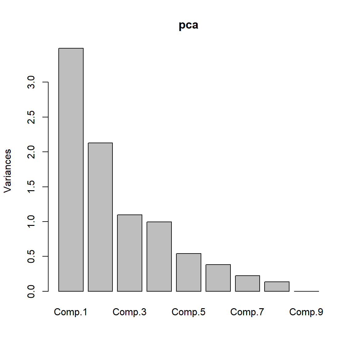
# PC1 and PC2 -- These are the weights of the variables on the first two Principal Components
pca$loadings[, 1:2]
#ans>       Comp.1  Comp.2
#ans> Agr  0.52379  0.0536
#ans> Min  0.00132  0.6178
#ans> Man -0.34750  0.3551
#ans> Pow -0.25572  0.2611
#ans> Con -0.32518  0.0513
#ans> Ser -0.37892 -0.3502
#ans> Fin -0.07437 -0.4537
#ans> Soc -0.38741 -0.2215
#ans> Tra -0.36682  0.2026
Based on the weights of the variables on the PCs shown above, we can extract the following interpretation:
- PC1 is roughly a linear combination of
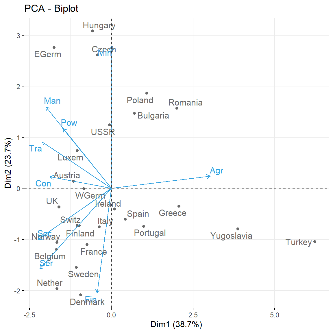
Agr, with negative weight, and (Man,Pow,Con,Ser,Soc,Tra), with positive weights. So it can be interpreted as an indicator of the kind of economy of the country: agricultural (negative values) or industrial (positive values). - PC2 has negative weights on (
Min,Man,Pow,Tra) and positive weights in (Ser,Fin,Soc). It can be interpreted as the contrast between relatively large or small service sectors. So it tends to be negative in communist countries and positive in capitalist countries.
The interpretation of the PCs involves inspecting the weights and interpreting the linear combination of the original variables, which might be separating between two clear characteristics of the data
To conclude, let’s see how we can represent our original data into a plot called biplot that summarizes all the analysis for two PCs.
# Biplot - plot together the scores for PC1 and PC2 and the
# variables expressed in terms of PC1 and PC2
biplot(pca)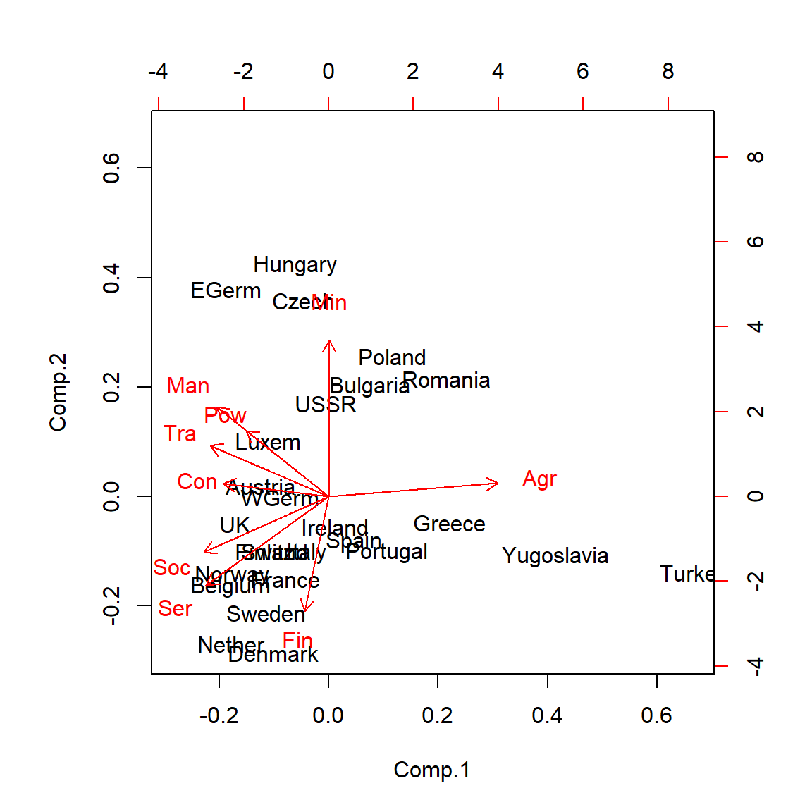
This biplot confirms the above interpretation.
Recall that the biplot is a superposition of two figures: the first one is the scatterplot of the principal component scores (the projections of the observations on the new low dimensional space - also know as graph of individuals) and the second one is the figure of loading vectors (also known as graph of variables). In fact, the graph of variables is a correlation circle, the variables whose unit vectors are close to each other are said to be positively correlated, meaning that their influence on the positioning of individuals is similar (again, these proximities are reflected in the projections of variables on the graph of individuals). However, variables far away from each other will be defined as being negatively correlated. Variables that have perpendicular unit vector are uncorrelated. To see both graphs we can use the factoextra package like follows:
# loading factoextra library
require(factoextra)
# Calculating pca using prcomp(), which is a built-in function in R
res.pca <- prcomp(eurojob, scale = TRUE)
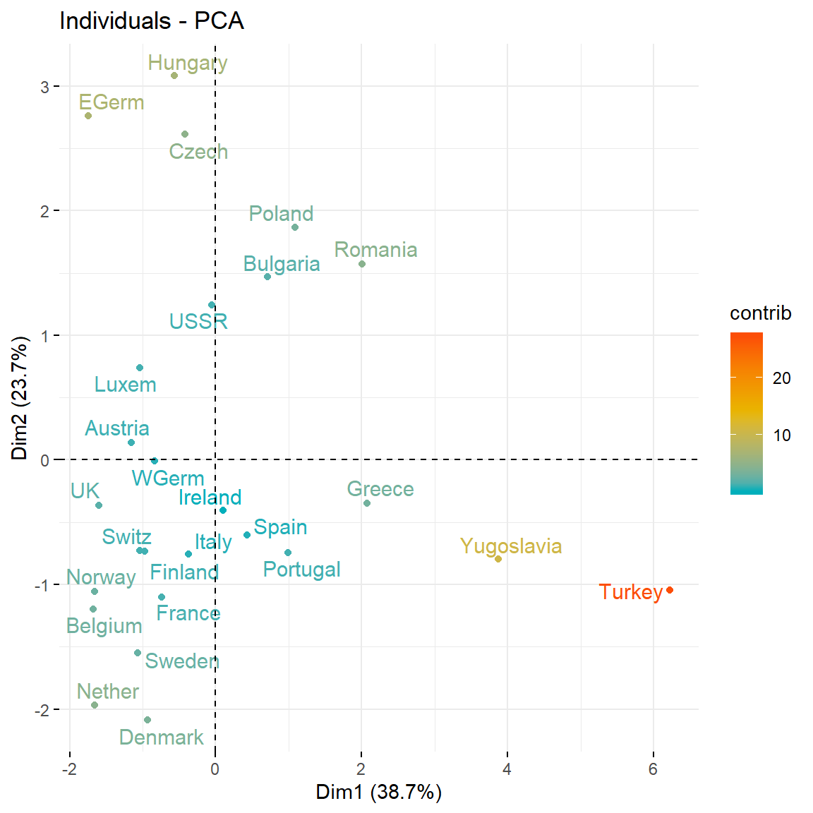
# Graph of individuals
fviz_pca_ind(res.pca,
col.ind = "contrib", # Color by their contribution to axes
gradient.cols = c("#00AFBB", "#E7B800", "#FC4E07"),
repel = TRUE
)
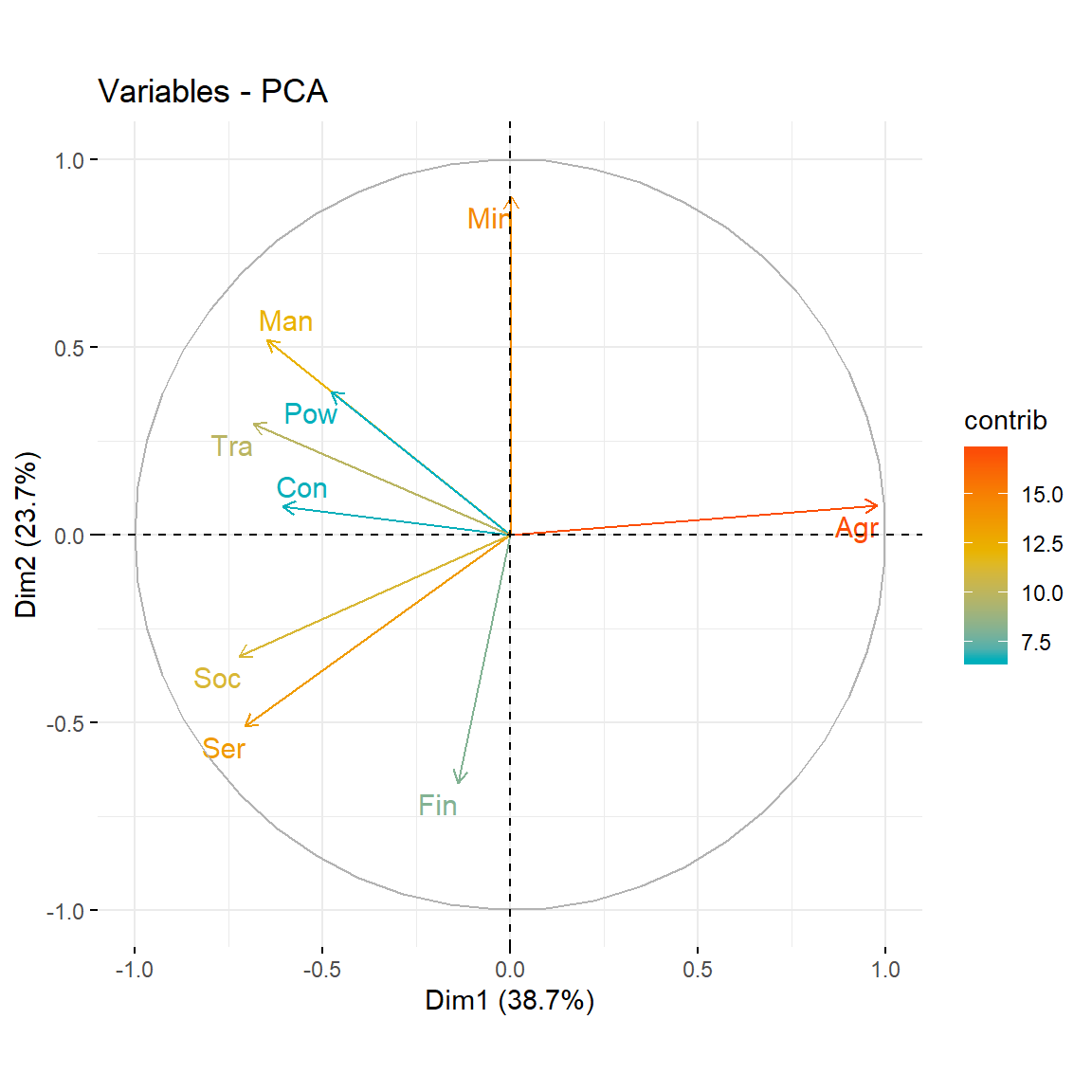
# Graph of variables
fviz_pca_var(res.pca,
             col.var = "contrib",
             gradient.cols = c("#00AFBB", "#E7B800", "#FC4E07"),
             repel = TRUE
             )
# Biplot of individuals and variables
fviz_pca_biplot(res.pca, repel = TRUE,
                col.var = "#2E9FDF",
                col.ind = "#696969"
                )
◼