9 Hierarchical Clustering
In the last two chapters we introduced \(k\)-means and Gaussian Mixture Models (GMM). One potential disadvantage of them is that they require us to prespecify the number of clusters/mixtures \(k\). Hierarchical clustering is an alternative approach which does not require that we commit to a particular choice of \(k\). Hierarchical clustering has an added advantage over \(k\)-means clustering and GMM in that it results in an attractive tree-based representation of the observations, called a dendrogram.
The most common type of hierarchical clustering is the agglomerative clustering (or bottom-up clustering). It refers to the fact that a dendrogram (generally depicted as an upside-down tree) is built starting from the leaves and combining clusters up to the trunk.
9.1 Dendrogram
Suppose that we have the simulated data in the following figure:
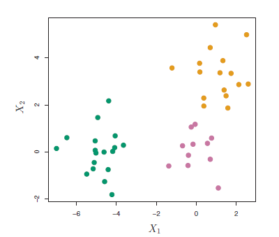
Figure 9.1: Simulated data of 45 observations generated from a three-class model.
The data in the figure above consists of 45 observations in two-dimensional space. The data were generated from a three-class model; the true class labels for each observation are shown in distinct colors. However, suppose that the data were observed without the class labels, and that we wanted to perform hierarchical clustering of the data. Hierarchical clustering (with complete linkage, to be discussed later) yields the result shown in Figure 9.2. How can we interpret this dendrogram?
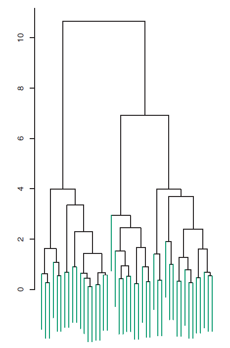
Figure 9.2: Dendrogram
In the dendrogram of Figure 9.2, each leaf of the dendrogram represents one of the 45 observations. However, as we move up the tree, some leaves begin to fuse into branches. These correspond to observations that are similar to each other. As we move higher up the tree, branches themselves fuse, either with leaves or other branches. The earlier (lower in the tree) fusions occur, the more similar the groups of observations are to each other. On the other hand, observations that fuse later (near the top of the tree) can be quite different. In fact, this statement can be made precise: for any two observations, we can look for the point in the tree where branches containing those two observations are first fused. The height of this fusion, as measured on the vertical axis, indicates how different the two observations are. Thus, observations that fuse at the very bottom of the tree are quite similar to each other, whereas observations that fuse close to the top of the tree will tend to be quite different.
An example of interpreting a dendrogram is presented in Figure 9.3
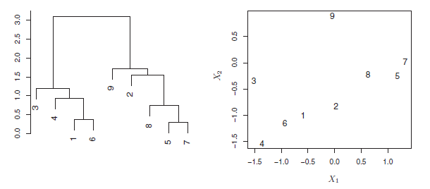
Figure 9.3: An illustration of how to properly interpret a dendrogram with nine observations in two-dimensional space. Left: a dendrogram generated using Euclidean distance and complete linkage. Observations 5 and 7 are quite similar to each other, as are observations 1 and 6. However, observation 9 is no more similar to observation 2 than it is to observations 8, 5, and 7, even though observations 9 and 2 are close together in terms of horizontal distance. This is because observations 2, 8, 5, and 7 all fuse with observation 9 at the same height, approximately 1.8. Right: the raw data used to generate the dendrogram can be used to confirm that indeed, observation 9 is no more similar to observation 2 than it is to observations 8, 5, and 7.
Now that we understand how to interpret the dendrogram of Figure 9.2, we can move on to the issue of identifying clusters on the basis of a dendrogram. In order to do this, we make a horizontal cut across the dendrogram, as shown in the following Figure 9.4 where we cut the dendro4 at a height of nine results in two clusters.
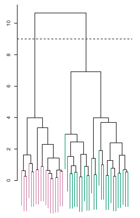
Figure 9.4: The dendrogram from the simulated dataset, cut at a height of nine (indicated by the dashed line). This cut results in two distinct clusters, shown in different colors.
The distinct sets of observations beneath the cut can be interpreted as clusters. In Figure 9.5, cutting the dendrogram at a height of five results in three clusters.
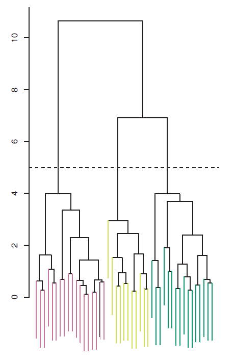
Figure 9.5: The dendrogram from the simulated dataset, cut at a height of five (indicated by the dashed line). This cut results in three distinct clusters, shown in different colors.
The term hierarchical refers to the fact that clusters obtained by cutting the dendrogram at a given height are necessarily nested within the clusters obtained by cutting the dendrogram at any greater height.
9.2 The Hierarchical Clustering Algorithm
The hierarchical clustering dendrogram is obtained via an extremely simple algorithm. We begin by defining some sort of dissimilarity measure between each pair of observations. Most often, Euclidean distance is used. The algorithm proceeds iteratively. Starting out at the bottom of the dendrogram, each of the n observations is treated as its own cluster. The two clusters that are most similar to each other are then fused so that there now are \(n−1\) clusters. Next the two clusters that are most similar to each other are fused again, so that there now are \(n − 2\) clusters. The algorithm proceeds in this fashion until all of the observations belong to one single cluster, and the dendrogram is complete.
Figure 9.6 depicts the first few steps of the algorithm.
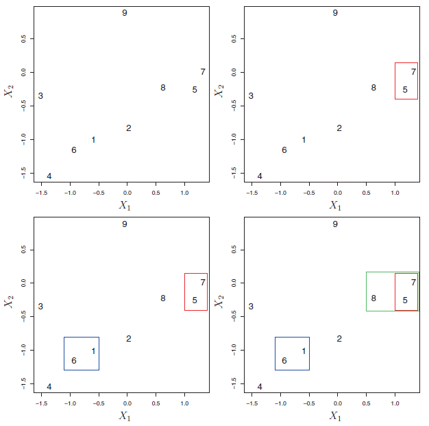
Figure 9.6: An illustration of the first few steps of the hierarchical clustering algorithm, with complete linkage and Euclidean distance. Top Left: initially, there are nine distinct clusters {1}, {2}, …, {9}. Top Right: the two clusters that are closest together, {5} and {7}, are fused into a single cluster. Bottom Left: the two clusters that are closest together, {6} and {1},are fused into a single cluster. Bottom Right: the two clusters that are closest together using complete linkage, {8} and the cluster {5, 7}, are fused into a single cluster.
To summarize, the hierarchical clustering algorithm is given in the following Algorithm:
| Hierarchical Clustering: |
| 1- Initialisation: Begin with \(n\) observations and a measure (such as Euclidean distance) of all the \(C^2_n = n(n−1)/2\) pairwise dissimilarities. Treat each observation as its own cluster. |
| 2- For \(i=n,n-1,\ldots,2\): |
| (a) Examine all pairwise inter-cluster dissimilarities among the \(i\) clusters and identify the pair of clusters that are least dissimilar (that is, most similar). Fuse these two clusters. The dissimilarity between these two clusters indicates the height in the dendrogram at which the fusion should be placed. |
| (b) Compute the new pairwise inter-cluster dissimilarities among the \(i − 1\) remaining clusters. |
This algorithm seems simple enough, but one issue has not been addressed. Consider the bottom right panel in Figure 9.6. How did we determine that the cluster {5, 7} should be fused with the cluster {8}? We have a concept of the dissimilarity between pairs of observations, but how do we define the dissimilarity between two clusters if one or both of the clusters contains multiple observations? The concept of dissimilarity between a pair of observations needs to be extended to a pair of groups of observations. This extension is achieved by developing the notion of linkage, which defines the dissimilarity between two groups of observations. The four most common types of linkage: complete, average, single, and centroid are briefly are described like follows:
Complete: Maximal intercluster dissimilarity. Compute all pairwise dissimilarities between the observations in cluster A and the observations in cluster B, and record the largest of these dissimilarities.
Single: Minimal intercluster dissimilarity. Compute all pairwise dissimilarities between the observations in cluster A and the observations in cluster B, and record the smallest of these dissimilarities. Single linkage can result in extended, trailing clusters in which single observations are fused one-at-a-time
Average: Mean intercluster dissimilarity. Compute all pairwise dissimilarities between the observations in cluster A and the observations in cluster B, and record the average of these dissimilarities.
Centroid: Dissimilarity between the centroid for cluster A (a mean vector of length p) and the centroid for cluster B. Centroid linkage can result in undesirable inversions.
Average and complete linkage are generally preferred over single linkage, as they tend to yield more balanced dendrograms. Centroid linkage is often used in genomics.
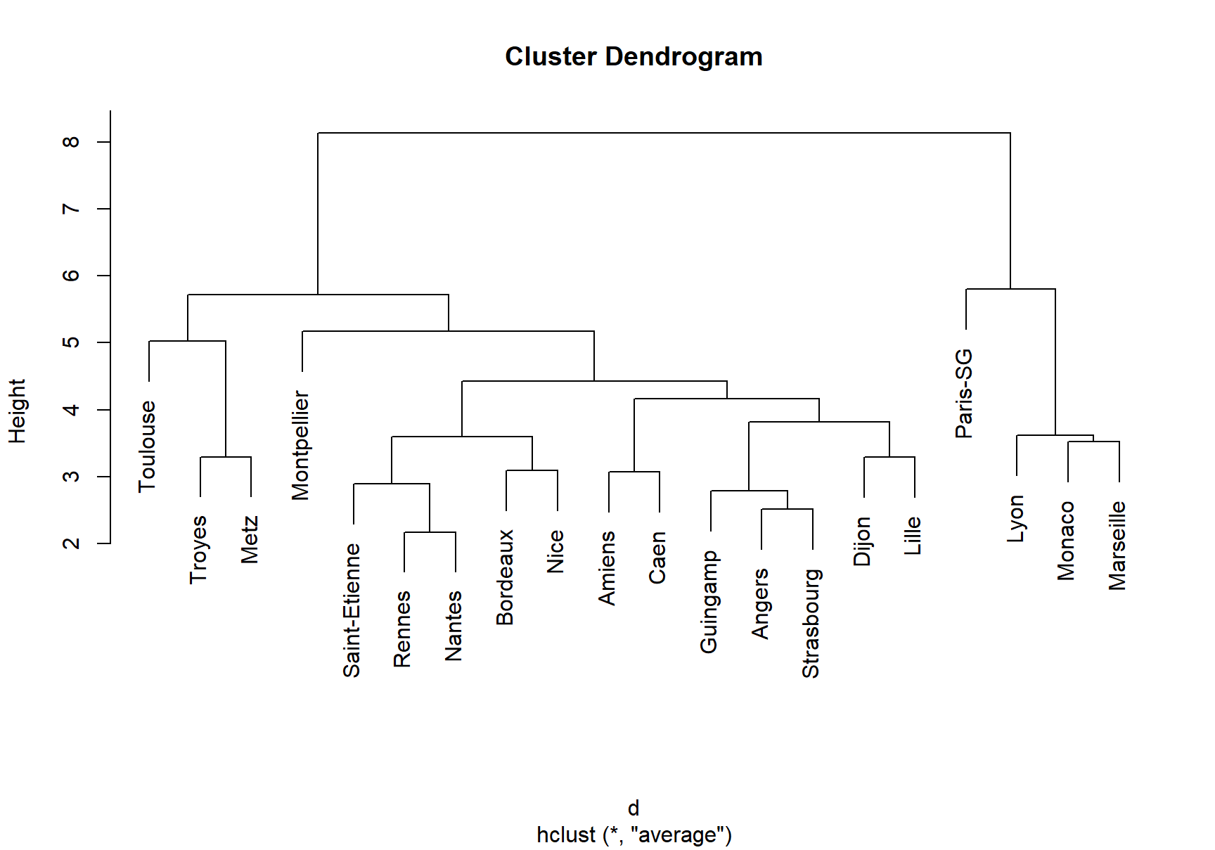
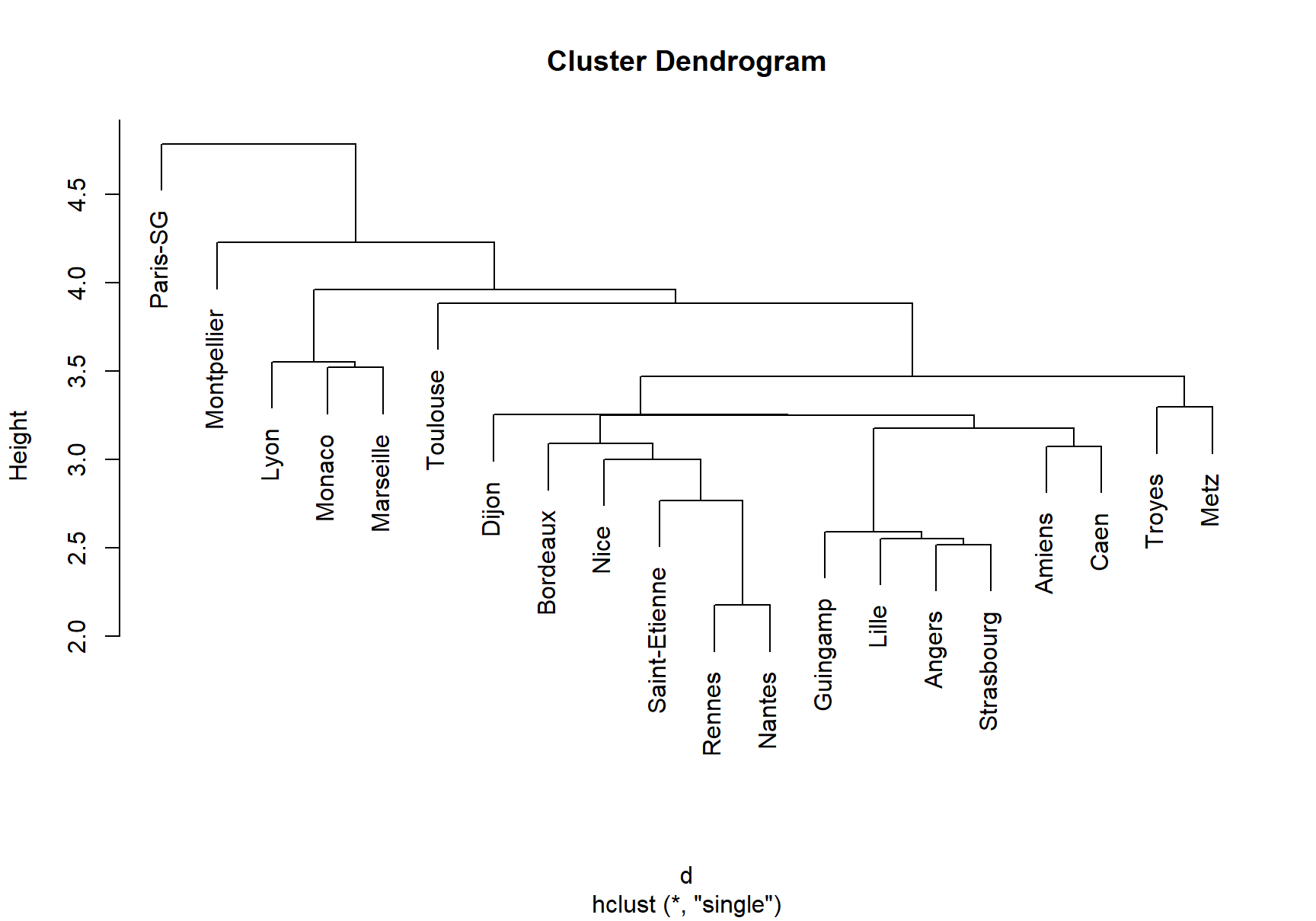
The dissimilarities computed in Step 2(b) of the hierarchical clustering algorithm will depend on the type of linkage used, as well as on the choice of dissimilarity measure. Hence, the resulting dendrogram typically depends quite strongly on the type of linkage used, as is shown in Figure 9.7.
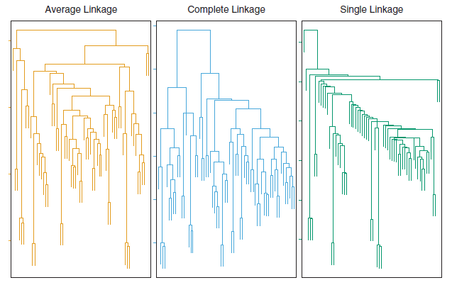
Figure 9.7: Average, complete, and single linkage applied to an example data set. Average and complete linkage tend to yield more balanced clusters.
9.3 Hierarchical clustering in R
Let’s illustrate how to perform hierarchical clustering on dataset Ligue1 2017-2018 .
# Load the dataset
ligue1 <- read.csv("datasets/ligue1_17_18.csv", row.names=1,sep=";")

# Work with standardized data
ligue1_scaled <- data.frame(scale(ligue1))

# Compute dissimilary matrix - in this case Euclidean distance
d <- dist(ligue1_scaled)

# Hierarchical clustering with complete linkage
treeComp <- hclust(d, method = "complete")
plot(treeComp)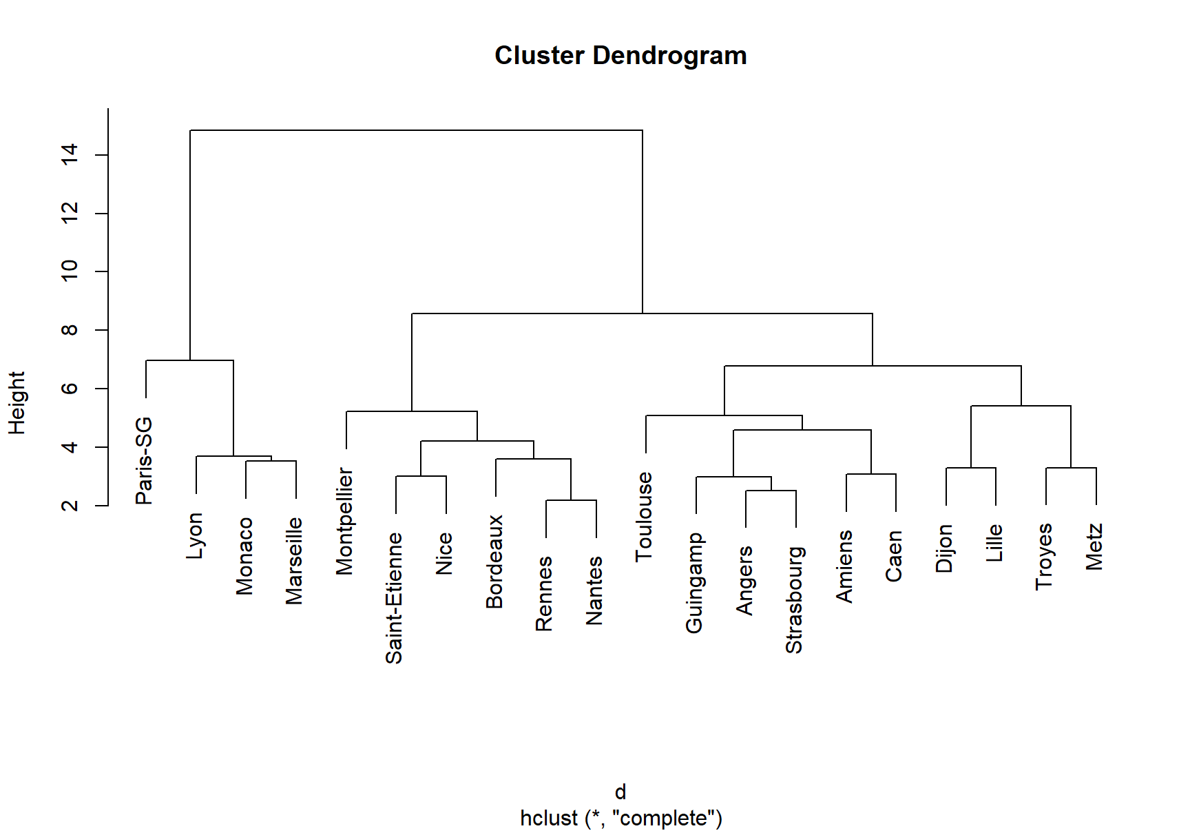
# Set the number of clusters after inspecting visually
# the dendogram for "long" groups of hanging leaves
# These are the cluster assignments
cutree(treeComp, k = 2) # (Barcelona, Real Madrid) and (rest)
#ans>      Paris-SG        Monaco          Lyon     Marseille        Rennes
#ans>             1             1             1             1             2
#ans>      Bordeaux Saint-Etienne          Nice        Nantes   Montpellier
#ans>             2             2             2             2             2
#ans>         Dijon      Guingamp        Amiens        Angers    Strasbourg
#ans>             2             2             2             2             2
#ans>          Caen         Lille      Toulouse        Troyes          Metz
#ans>             2             2             2             2             2
cutree(treeComp, k = 3) # (Barcelona, Real Madrid), (Atlético Madrid) and (rest)
#ans>      Paris-SG        Monaco          Lyon     Marseille        Rennes
#ans>             1             1             1             1             2
#ans>      Bordeaux Saint-Etienne          Nice        Nantes   Montpellier
#ans>             2             2             2             2             2
#ans>         Dijon      Guingamp        Amiens        Angers    Strasbourg
#ans>             3             3             3             3             3
#ans>          Caen         Lille      Toulouse        Troyes          Metz
#ans>             3             3             3             3             3
# Compare differences - treeComp makes more sense than treeAve
cutree(treeComp, k = 4)
#ans>      Paris-SG        Monaco          Lyon     Marseille        Rennes
#ans>             1             2             2             2             3
#ans>      Bordeaux Saint-Etienne          Nice        Nantes   Montpellier
#ans>             3             3             3             3             3
#ans>         Dijon      Guingamp        Amiens        Angers    Strasbourg
#ans>             4             4             4             4             4
#ans>          Caen         Lille      Toulouse        Troyes          Metz
#ans>             4             4             4             4             4
◼